


7.8: Parallelism: Using the MPI backend
This example demonstrates how to use the MPI backend for simulating
dipoles using hnn_core.
hnn_core can take advantage of MPI libraries such as OpenMPI to run a
single simulation using multiple CPU
processors. MPI lets you divide parts of your simulated network across
CPUs while allowing the CPUs to "talk" to each other, and can therefore
enable significant speed-up of individual simulations.
Note that to use MPI parallelism, you need either the
conda install or the pip
MPI Installation dependencies described in
our Installation Guide here.
Note that MPI parallelism is distinct from hnn_core's
use of Joblib
parallelism, which can be found here.
Authors:
- Mainak Jas ( mjas@mgh.harvard.edu )
- Blake Caldwell ( blake_caldwell@brown.edu )
- Austin Soplata ( austin_soplata@brown.edu )
1. Import MPI dependencies
Please note that in order to run this tutorial you MUST have installed HNN-Core with MPI support, which requires multiple steps. Normally, this is optional for general HNN-Core use, but it is required for this tutorial. In the next cell, we will check to make sure MPI support is installed, and if it is not, then please follow the directions provided.
                        try:
    import mpi4py  : F401
except ModuleNotFoundError:
    raise ModuleNotFoundError(
        "MPI parallelism for HNN-Core has not been installed correctly. "
        "Please follow the directions for installing MPI support at \n" \
        "\n" \
        " https://jonescompneurolab.github.io/textbook/content/01_getting_started/installation.html \n" \
        "\n" \
        "The easiest way to install HNN-Core with MPI support is to use the `conda Package Installation` method described in the link above."
    ) from None
After following the above instructions, we should be able to import
MPIBackend with full parallelism support.
from hnn_core import MPIBackend
2. Import other dependencies
Let us import what else we need from hnn_core and
matplotlib:
                        import matplotlib.pyplot as plt

from hnn_core import simulate_dipole, neymotin_2020_model
from hnn_core.viz import plot_dipole
3. Setup our network
Following our Alpha example, we will create our network and add a ~10 Hz "bursty" drive:
                        net = neymotin_2020_model()

weights_ampa = {'L2_pyramidal': 5.4e-5, 'L5_pyramidal': 5.4e-5}
net.add_bursty_drive(
    'bursty', tstart=50., burst_rate=10, burst_std=20., numspikes=2,
    spike_isi=10, n_drive_cells=10, location='distal',
    weights_ampa=weights_ampa, event_seed=278)
4. Simulate using MPIBackend
Finally, we will simulate using the MPIBackend
class. This will start the simulation across the number of
processors (cores) specified by n_procs using MPI.
                    with MPIBackend(n_procs=4, mpi_cmd='mpiexec'):
dpls = simulate_dipole(net, tstop=210., n_trials=1)
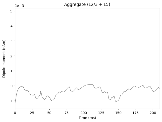
5. Visualize our output
Having used MPIBackend, our simulation should have run
considerably faster than it would using only a single core,
approximately 4 times faster!
                        plot_dipole(dpls, show=False)
plt.show()