5.1 GUI Tutorial of Alpha/Beta Rhythms

Tutorial Table of Contents

1. Background

2. Downloading HNN Parameter Set Files

3. Setting Initial Simulation and Visualization Parameters

4. Simulating Rhythmic Proximal Inputs: Alpha only

5. Simulation Rhythmic Distal Inputs: Alpha only

6. Simulating Combined Rhythmic Proximal and Distal Inputs: Alpha/Beta Complex

7. Adjusting parameters

1. Background

In order to understand the workflow and initial parameter sets provided with this tutorial, we must first briefly describe prior studies that led to the creation of the data you will aim to simulate. This tutorial is based on results from (Stephanie R. Jones et al. 2009) where, using MEG, we recorded spontaneous (pre-stimulus) alpha (7-14 Hz) and beta (15-29 Hz) rhythms that arise as part of the mu-complex from the primary somatosensory cortex (S1) (Stephanie R. Jones et al. 2009). (Figure 1, See also (Ziegler et al. 2010), (Sherman et al. 2016), (Stephanie R. Jones 2016).)

Figure 1

Figure 1 Left: Spectrogram of spontaneous activity from current dipole source in SI averaged across 100 trials from an example subject. The spectrogram shows nearly continuous prestimulus alpha and beta oscillations. At time zero, a brief tap was given to the contralateral finger tip, causing the spontaneous oscillations to briefly desynchronize.

Figure 1 Right: A closer look at the prestimulus waveform and spectrogram from spontaneous activity during individual example signal trials. This illustrates that the alpha and beta oscillations occur intermittently and are frequently non-overlapping.

All figures in Figure 1 are from (Stephanie R. Jones et al. 2009) or related work.

Our goal was to use our neocortical model to reproduce features of the waveform and spectrogram observed on single (un-averaged) trials (Figure 1, middle and right columns), where the alpha and beta components emerge briefly and intermittently in time. On any individual trial (i.e., 1 second of spontaneous, pre-stimulus data), the presence of alpha and beta activity is not time-locked and is representative of so-called “induced” activity. The alpha and beta bands of activity appear continuous when averaging the spectrograms across trials (Figure 1, left column), but this is due to the fact that the spectrograms values are strictly positive and the alpha and beta events accumulate without cancellation (Stephanie R. Jones 2016). For individual trials, alpha and beta power is simultaneously high only around 50% of the time, as shown in Figure 2.

Figure 2

Figure 2: Key features of the spontaneous non-average SI alpha/beta complex include: intermittent transient bouts of alpha/beta activity, a waveform that oscillates around 0 nAm, power spectral densities (PSD) with peaks in the alpha and beta bands, primarily non-overlapping alpha and beta events, and a symmetric waveform oscillation. The model was able to reproduce each of these features. The subplots in the top row are from experimental MEG data exhibiting these features, while the corresponding subplots in the bottom row are from simulations of the model. See (Stephanie R. Jones et al. 2009).

We found that a sequence of exogenous subthreshold excitatory synaptic drive could activate the network in a manner that reproduced important features of the SI rhythms in the model (Figure 2). This drive consisted of two nearly-synchronous 10 Hz rhythmic drives that contacted the network through proximal and distal projection pathways (Figure 3, see also Textbook Section 2.5: Evoked and Rhythmic Driving Inputs). The drives were simulated as population “bursts” of action potentials that contacted the network every 100ms with the mean delay between the proximal and distal burst of 0ms. Specifically, as shown schematically in Figure 3, these 10 population bursts consisted of 2-spike bursts (i.e. spike “doublets”), Gaussian distributed in time. We presumed that during such spontaneous activity, these drives may be provided by leminscial and non-lemniscal thalamic nuclei, which contact proximal and distal pyramidal neurons respectively, and they are know to burst fire at ~10 Hz frequencies in spontaneous states ((E. G. Jones 2001), (Hughes and Crunelli 2005)).

Figure 3

Figure 3: Schematic illustration of exogenous 10 Hz burst drives through proximal and distal projection pathways. “Population bursts”, consisting of a set number of “burst units” (10 instances of 2-spike bursts as shown) drive post-synaptic conductances in the local network with a set frequency (100 ms inter-burst-interval, equal to 10 Hz) and a variable mean delay between proximal and distal drives.

We assumed that the macroscale rhythms generating the observed alpha and beta activity arose from subthreshold current flow in a large population of neurons, as opposed to being generated by local spiking interaction (Zhu et al. 2009). As such, the effective strengths of the exogenous driving inputs were tuned so that the cells in the network remained subthreshold (all other parameters were tuned and fixed based on the morphology, physiology, and connectivity within layered neocortical circuits, see (Stephanie R. Jones et al. 2009) for details). The inputs drove subthreshold currents up (proximal) and down (distal) the pyramidal neurons in order to reproduce accurate waveform and spectrogram features (see Figure 3). A scaling factor of 3000 was multiplied by the model waveform to reproduce a signal in units of nAm, comparable to the recorded data, suggesting that on the order of 200 x 3000 = 600,000 pyramidal neurons contributed to this signal.

We further found that increasing the strength and synchrony of the distal drive created stronger beta activity, but increasing the delay between the drives to ~50ms created a pure alpha oscillation (see Section 7 below). The former result led to the novel prediction that brief beta events emerge when a broad proximal drive is disrupted by a simultaneous strong distal drive lasting 50ms (i.e., one beta period). Support for this prediction was found invasively with laminar recordings in mice and monkeys (Sherman et al. 2016).

In this tutorial, we will explore parameter changes that illustrate these results. We will walk you step-by-step through simulations with various combinations of rhythmic proximal and distal drives to describe how each contributes to the alpha and beta components of the SI alpha/beta complex. We will not be simulating evoked responses or how alpha/beta oscillations interact with evoked responses; click here for our GUI tutorial on simulating evoked-response potentials (ERPs).

We will begin by simulating only rhythmic proximal 10 Hz inputs (Section 4), followed by simulating only distal 10 Hz inputs (Section 5), followed by various combinations of proximal and distal drives to generate combinations of alpha and beta rhythms (Section 6). We’ll show you how HNN can plot waveforms, time-frequency spectrograms, and power spectral density plots of the simulated data.

2. Downloading HNN Parameter Set Files

Throughout this tutorial, we will be using several different HNN parameter set files. These files are not included in the HNN installation, but instead must be downloaded separately, similar to the files you downloaded in the Morning session of the workshop. The easiest way to get them is to click this link, which will download a ZIP file that contains the four files we need. Alternatively, you can download (or git clone) this Github repository: hnn-data and then access the files in the workshops/alpha_beta_gui_walkthrough directory. These four files are named OnlyRhythmicProx.json, OnlyRhythmicDist.json, AlphaAndBeta.json, and AlphaAndBetaJitter50.json.

Begin by starting the HNN GUI. If you are using Google Colab notebook, follow the instructions there for starting and accessing the GUI. If you are using a local install of HNN, run the following command from a terminal:

hnn-gui

3. Setting Initial Simulation and Visualization Parameters

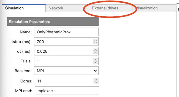
Before running any simulations, we need to change some default parameters of both the simulations and visualizations. The parameters we need to change in the Simulation tab are shown in Figure 4 below, and are also listed below. Please note that if you refresh the browser tab or restart HNN, you will have to re-enter all of these parameter changes.

1. Change the Name of the simulation to OnlyRhythmicProx (or you can change it to whatever you prefer).
2. Change tstop (ms) to 700. This will increase the length of the simulation to 700 milliseconds, and enable us to see simulated oscillations as they evolve over longer time periods.
3. Change Dipole Smoothing to 0.
4. Change Min Spectral Frequency (Hz) to 5.
5. Change Max Spectral Frequency (Hz) to 40. These two changes will make it easier to see the alpha and beta frequency ranges.
6. Only if you are using Mac or Linux (not Windows), and only if you installed HNN locally using the instructions provided on the Workshop page, then do the following (you may have already obtained this number in the initial install):
   1. run the following command in a Terminal: python -c "import psutil ; print(psutil.cpu_count(logical=False)-1)"
   2. read the output number,
   3. put that number in the Cores textbox of the GUI. This will greatly increase your simulation speed.

Figure 4

4. Simulating Rhythmic Proximal Inputs: Alpha Only

4.1 Load and view our proximal inputs

As described in Section 1. Background, low-frequency alpha and beta rhythms can be simulated by a combination of rhythmic subthreshold proximal and distal ~10Hz inputs. Here, we begin by describing the impact of only proximal inputs. An initial parameter set that will simulate the effect of ~10 Hz subthreshold proximal drive is provided in the file OnlyRhythmicProx.json, which you downloaded in Section 2

The default cortical column network for this simulation, and HNN as a whole, is described in the Template Model section. Several of the network parameters can be adjusted via the GUI in the Network tab (e.g. local excitatory and inhibitory connection strengths), but we will not be changing them in this tutorial. Instead, we will only be changing parameters in the Simulation, External drives, and Visualization tabs.

To load the initial parameter set, navigate to the GUI and do the following steps (these are illustrated below in Figure 5):

1. Click the tab labeled: External drives.
2. Inside of the inside of the tab, click the button Load external drives (0), then select the file OnlyRhythmicProx.json, which you downloaded previously in Section 2.
3. To view the parameters that “activate” the network via rhythmic proximal input, click the dropdown menu labeled bursty1 (proximal).

You should now be able to scroll and see the values of adjustable parameters, displayed as in the dialog boxes below in Figure 6. There are 4 sections, which we will describe in greater detail below. For now, we will not change any of these parameters, but instead only describe them.

1. bursty1 (proximal): The first section deals with all properties of the drive not included in other sections, including the timing settings, statistical properties, number of spikes per burst, number of virtual “drive cells”, and pseudo-random number generation seed. This is an important section which we will return to frequently.
2. AMPA weights: This section governs the excitatory AMPAergic post-synaptic conductances from the drive onto the excitatory Layer 5 and Layer 2/3 Pyramidal cells, and onto inhibitory Layer 5 and Layer 2/3 Basket cells. All synapse conductances are given in units of microSiemens, or $\mu S$.
3. NMDA weights: which is analagous to the AMPA weights section, but for the NMDA synapses.
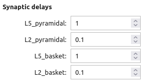
4. Synaptic delays: This section governs the synaptic delays from the drive to all cell types.

Rhythmic proximal input occurs through stochastic, presynaptic bursts of action potentials from a population of bursting cells onto postsynaptic neurons of the modelled network (see Figure 3). All drive stochasticity is controlled by parameters in the first section of these four. The spike train start time for each bursting cell is sampled from a normal distribution with mean Start time (ms) and standard deviation Start time dev (ms). The inter-burst intervals, or time between bursts, for each bursting cell are sampled from a normal distribution of mean $\frac{1}{BurstRate (Hz)}$ (e.g., a Burst rate (Hz) of 10 Hz corresponds to an inter-burst interval of 0.1 second or 100 ms) and standard deviation Burst std dev (Hz) (see Figure 3). Also note that the number of spikes per burst unit is set with No. Spikes and the final stop time for the entire population of rhythmic proximal inputs is set with Stop time (ms).

For more discussion on the rhythmic drive model itself, see Model Assumptions: 2.5 Evoked and Rhytymic Driving Inputs.

4.2 Run the simulation and visualize the net current dipole

To run this simulation, navigate to the main GUI window and click:

Run

This simulation runs for 700 ms of simulation time, so will take longer to run than the ERP simulations in the Morning session. Each of the individual simulations in this tutorial will take approximately 4 minutes to run using the Google CoLab notebook. Once completed, you will see output similar to that shown below.

Figure 7

Concerning stochasticity: As shown in the red histogram in the top panel of Figure 7 above, with this parameter set, a burst of proximal input spikes is provided to the network at a rate of ~10 Hz (i.e., every 100 ms). Due to the stochastic nature of the inputs (controlled by the Start time dev (ms) and Burst std dev (Hz) parameters), there is some variability in the histogram of proximal input times, and the exact histogram pattern may look different on your simulation. Note that a decrease in the Burst std dev (Hz) would create shorter duration bursts (i.e., more synchronous bursts); this will be explored further in Section 6.2 below.

The main point with this simulation is that ~10 Hz bursts of proximal drive induce current flow up the pyramidal neuron dendrites. This upward current flow increases the dipole signal above the 0 nAm baseline (making it positive), before the dipole relaxes back to zero approximately every 100 ms. This is observed in the blue current dipole waveform in the GUI window. See Figure 3 and Figure A on the Workshop page for illustration of the relationship between proximal drive input and the flow of current.

4.3 Visualize the spectrogram of the net current dipole

To view the time-frequency spectrogram for this waveform (shown below in Figure 8), do the following steps:

1. Click on the Visualization tab.
2. Click on the Layout template dropdown menu and select Drive-Dipole-Spectrogram (3x1).
3. Click on the Dataset dropdown menu and select the most recent simulation name, which is OnlyRhythmicProx (or whatever you set the Name to previously).
4. Finally, click the Make Figure button.

Figure 8

The bottom panel of Figure 8 shows the corresponding time-frequency spectrogram for this waveform, which exhibits a high-power continuous 10 Hz signal.

Importantly, in this example, the strength of the proximal input spikes were titrated to be subthreshold. In other words, our simulated cortical cells do not spike in this instance. This is because we assume that macroscale oscillations are generated primarily by subthreshold current flow across large populations of synchronous pyramidal neurons (see Section 1. Background above for details). We will illustrate the relationship between spiking and the signal later, in Section 6.3 (see also our ERP tutorial).

This exploration with a proximal drive is only useful in understanding how subthreshold rhythmic inputs impact the current dipole produced by the circuit. However, several features of the waveform and spectrogram of the signal do not match the recorded data shown in Figure 1 and Figure 2. Next, we explore the impact of rhythmic distal inputs only (Section 5), and then a combination of the two (Section 6).

5. Simulation Rhythmic Distal Inputs: Alpha only

5.1 Load/view parameters to define the network structure & to “activate” the network

We will next use a param file that generates bursts of only distal inputs provided at the alpha frequency (10 Hz), file OnlyRhythmicDist.json. Do the folowing steps:

1. Click back to the Simulation tab.
2. Change the Name of the simulation to OnlyRhythmicDist (or whatever you prefer).
3. Click the tab labeled: External drives.
4. Inside of the inside of the tab, click the button Load external drives (0), then select the file OnlyRhythmicDist.json, which you downloaded previously in Section 2.
5. To view the parameters that “activate” the network via rhythmic distal input, click the dropdown menu labeled bursty2 (distal).

You should see the values of adjustable parameters displayed as in the dialog boxes below in Figure 9. Notice that these parameters are the same as those regulating the proximal drive in Section 4, except for the synaptic delays. In this case, the parameters define bursts of synaptic inputs that drive the network in a distal projection pattern, which are illustrated in Figure 3 and Figure A on the Workshop page.

To run this simulation, navigate to the main GUI window and click:

Start Simulation

Once completed, you will see output similar to that shown below.

Figure 10

As shown in the green histogram in the top panel of the HNN GUI above, with this parameter set, a burst of distal input spikes is provided to the network ~10 Hz (i.e., every 100 ms). As discussed previously, due to the stochastic nature of the inputs (controlled by the Start time dev (ms) and Burst std dev (Hz) parameters), there is some variability in the histogram of proximal input times.

The ~10 Hz bursts of distal input induces current flow down the pyramidal neuron dendrites, decreasing the signal below the 0 nAm baseline (making it negative), followed by the signal relaxing back to zero, approximately every 100 ms. This is observed in the blue current dipole waveform in the GUI window. Once again, see Figure 3 above and Figure A on the Workshop page for the relationship between distal inputs and direction of signal propagation.

Once again we will create time-frequency spectrogram for this waveform:

1. Click on the Visualization tab.
2. Click on the Layout template dropdown menu and select Drive-Dipole-Spectrogram (3x1).
3. Click on the Dataset dropdown menu and select the most recent simulation name, which is OnlyRhythmicDist (or whatever you set the Name to previously).
4. Finally, click the Make Figure button.

Figure 11

The bottom panel shows the corresponding time-frequency spectrogram for this waveform that exhibits a high power continuous 10 Hz signal. Importantly, in this example, the strength of the distal input was also titrated to be subthreshold (i.e., cells do not spike). Again, ee will illustrate the relationship between spiking and the signal later, in Section 6.3 (see also our ERP tutorial).

While instructional, this simulation also does not produce waveform and spectral features that match the experimental data in Figure 1 and Figure 2. In the next section (Section 6), we describe how combining both the 10 Hz proximal and distal drives can produce an oscillation with many characteristic features of the spontaneous SI signal (Stephanie R. Jones et al. 2009).

6. Simulating Combined Rhythmic Proximal and Distal Inputs: Alpha/Beta Complex

6.1 Load/view parameters to define the network structure & to “activate” the network.

In this example, we provide a parameter set file AlphaAndBeta.json that produces many of the waveform and spectral features observed in our SI data (Figure 2).

1. Click back to the Simulation tab.
2. Change the Name of the simulation to AlphaAndBeta
3. Click the tab labeled: External drives.
4. Inside of the inside of the tab, click the button Load external drives (0), then select the file AlphaAndBeta.json, which you downloaded previously in Section 2.
5. To view the parameters that “activate” the network via rhythmic distal input, click the dropdown menus labeled bursty1 (proximal) and bursty2 (distal).

You should see the values displayed in the dialogue boxes below.

Figure 12

In this simulation, all external drive parameters the same as they were for each drive in the previous simulations (except for the random Seed). The only significant difference is that both distal and proximal drives are included.

Importantly, the Start time (ms) values for both inputs are set to 50.0 ms, meaning that the proximal and distal input bursts will arrive nearly synchronously to the network on each cycle of the 10 Hz input. However, due to the stochasticity in the parameters (Start time dev (ms) and Burst std dev (Hz)), sometimes the bursts will arrive together and sometimes there will be a slight delay. As will be described further below, this stochasticity will create intermittent alpha and beta events.

6.2 Run the simulation and visualize net current dipole

To run this simulation, navigate to the main GUI window by clicking the Simulation tab and then click:

Run

Once completed, you will see output similar to that shown below.

Figure 13

Follow the steps in the previous sections (such as Section 4.3) to create a time-frequency spectrogram for this waveform, and remember to set Dataset to the most recent simulation, AlphaAndBeta. The output will look similar to the figure below:

Figure 14

As shown in the green and red histogram in the top panel of the GUI Figures above, with this parameter set, bursts of both proximal and distal input spikes are provided to the network ~10 Hz (i.e., every 100 ms). Due to the stochastic nature of the inputs, there is some variability in the timing and duration of the input bursts: sometimes they arrive at the same time, and sometimes there is a slight offset between them. As a result, intermittent, transient alpha and beta events emerge in the time-frequency spectrogram.

Alpha events are produced when the inputs occur slightly out of phase and current flow is pushed alternately up and down the dendrites for ~50 ms duration each; the current flow of either burst input type does not interfere with the other. Beta events, in contrast, occur when the burst inputs arrive more synchronously; this causes upward current flow to be disrupted by downward current flow for ~50 ms, effectively cutting the oscillation period in half. Therefore, the relative expression of alpha versus beta can be controlled by the relative delay between the inputs and their relative burst strengths.

The current dipole signal of this simulation, shown in the above figure, oscillates above and below 0 nAm, which qualitatively matches the experimental data (see Figure 1 and Figure 2 in Section 1. Background). This is different than the proximal- or distal-only simulations in prior sections, since the current in the pyramidal neurons is pushed both upward and downward in this simulation. Additionally, this simulation reproduces the transient nature of the alpha and beta activity and several other features of the waveform and spectrogram can be quantified to show close agreement between model and experimental results (see Figure 2 above, and (Stephanie R. Jones et al. 2009) for further details).

We note that here, we do not directly compare the spontaneous current dipole waveform to recorded data, as is done in the ERP tutorial with a root mean squared error. This is due to the fact that the spontaneous SI signal we are simulating is not time-locked to alpha or beta events on any given trial, and the stochastic nature of the driving inputs causes variability in the timing of the alpha or beta activity, making it difficult to align recorded data and simulated results.

6.3 Viewing network spiking activity

Importantly, in all the simulations of this tutorial so far, the strength of the proximal and distal inputs were titrated to be subthreshold, meaning that they do not cause our simulated cortical cells to spike. This is based on our assumption that macroscale oscillations are generated primarily by subthreshold current flow across large populations of synchronous pyramidal neurons (see Section 1. Background for references). We can verify the subthreshold nature of the inputs by viewing the spiking activity in the network. Do the following steps to see our spiking rastergram:

1. Click on the Visualization tab.
2. Click on the Layout template dropdown menu and select Drive-Spikes (2x1).
3. Click on the Dataset dropdown menu and select the most recent simulation name, which is AlphaAndBeta.
4. Finally, click the Make Figure button.

Figure 20

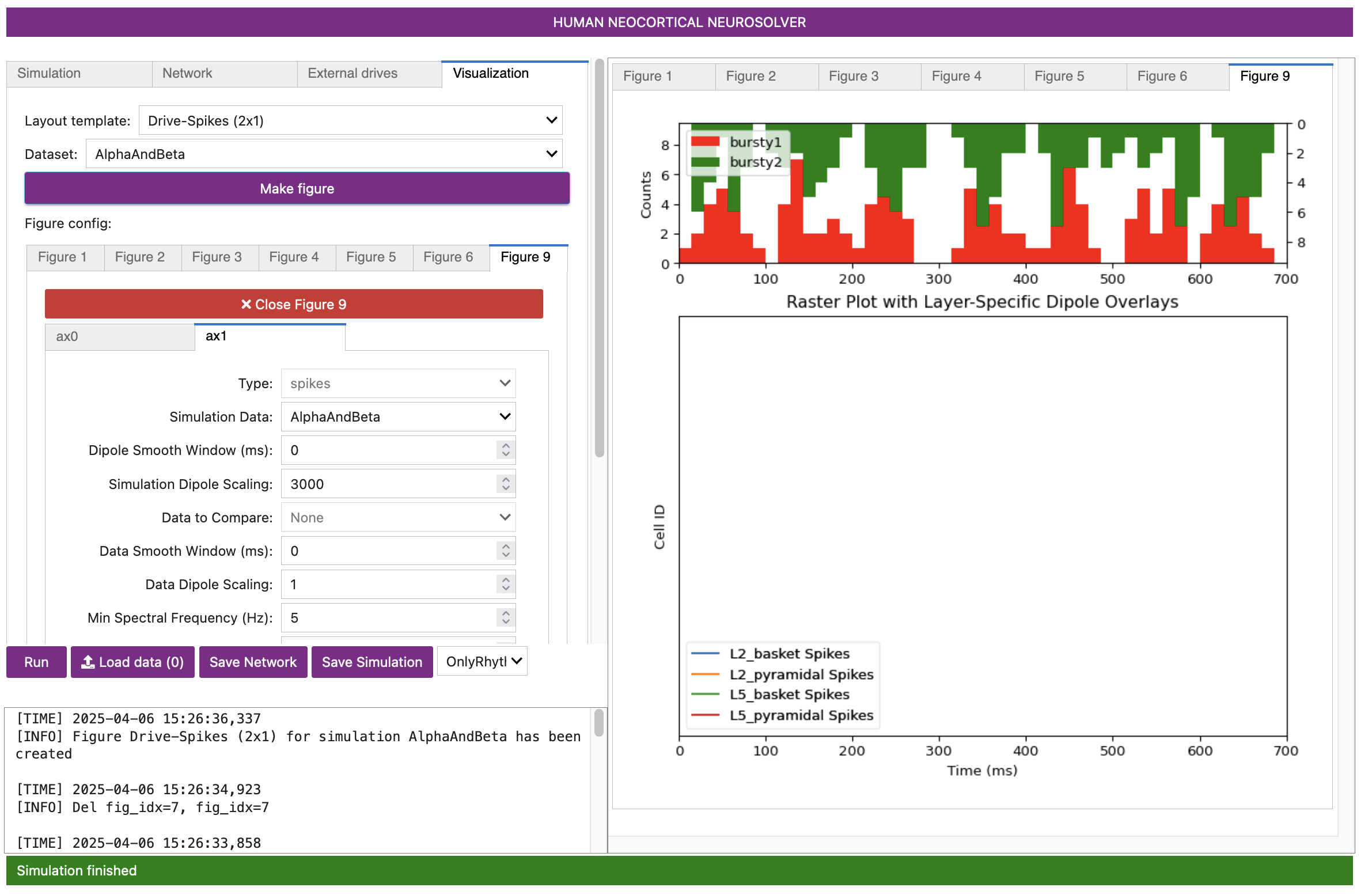
In this window, the rhythmic distal (green/top) and proximal (red/middle) input-burst-histograms are shown above the spiking activity in each population of cells (bottom panel). In this case, the alpha and beta events are indeed produced through subthreshold processes, and there is no spiking produced in any cell in the network (i.e. there are no dots present in the bottom raster plot)!

6.4 Simulating and averaging multiple trials with jittered start times creates the impression of continuous oscillations

As described in Section 1. Background above, our simulation goal was to study the mechanisms that reproduce features of spontaneous alpha and beta rhythms observed in un-averaged data. These features include the fact that alpha and beta components are transient and intermittent (Figure 1, right panel). Each tutorial section up to this point was based on simulating un-averaged data.

Here, we will show that, depending on the stochastic nature of the proximal and distal rhythmic inputs, alpha and beta activity on different simulation “trial” may be jittered, creating the impression of continuous oscillations. We will describe how to run and average multiple simulation “trials” (700 ms epochs of spontaneous activity), and change the stochasticity by changing the standard deviation of the start times of the drives (Start time dev (ms)). This is akin to simulating induced rhythms rather than time-locked evoked rhythms. In the averaged spectrogram across trials, the alpha and beta events will accumulate without cancellation (due to the fact that spectrogram values are purely positive), creating the impression of a continuous oscillation, such as in Figure 1.

1. Click back to the Simulation tab.
2. Change the Name of the simulation to AlphaAndBetaJitter50
3. Click the tab labeled: External drives.
4. Inside of the inside of the tab, click the button Load external drives (0), then select the file AlphaAndBetaJitter50.json, which you downloaded previously in Section 2.
5. To view the parameters that “activate” the network via rhythmic distal input, click the dropdown menus labeled bursty1 (proximal) and bursty2 (distal).

You should see the values displayed in the dialogue boxes below.

For this simulation, the only difference in the parameters from that of the prior AlphaAndBeta.json simulation is that Start time dev (ms) for both drives has been increased from 0 to 50 ms. Both drives will still input at a 10 Hz rate, but the distal versus proximal inputs are less likely to occur at the same time.

Finally, we need to change one more parameter before we run the simulations: Trials. If we increase Trials above 1, this will cause HNN to run that number of consecutive simulations, each with different randomized initial conditions for the drives. After all trial simulations are complete, the averaged data will automatically be computed and plotted. You will then be able to do further plots using the averaged signal. Note that increasing the number of trials will correspondingly increase the amount of time needed to run the simulations; e.g. if you are using the Google Colab notebook, running 3 trials may take approximately 12 minutes if a single simulation takes 4 minutes. (We do support parallelization of simulation across trials, but this is beyond the scope of this tutorial; see our Joblib instructions here.)

Do the following:

1. Click back to the Simulation tab.
2. Change the Trials to 3.
3. Click Run.

Once completed, we recommend you immediately plot the spectrogram of these simulations, using the instructions before in Section 4.3 and selecting the new dataset for AlphaAndBetaJitter50. You should get a plot that looks like below:

Figure 16

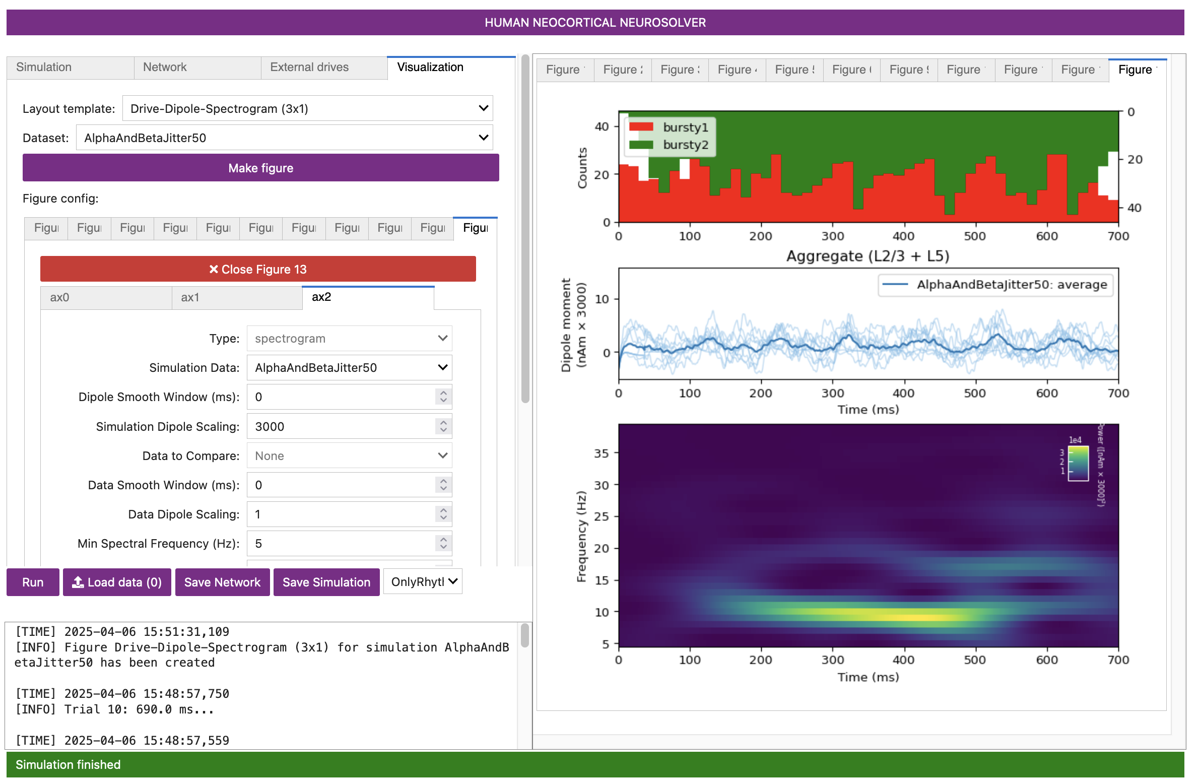
Notice that the input histograms for distal (green) and proximal (red) input accumulated across the 10 trials now show little rhythmicity due to the jitter in the rhythmic input start times across trials (Start time dev (ms) = 50), in addition to jitter due to the inherent burst variance (Burst std dev (Hz) = 20). However, if we were to visualize histograms on each individual trial, they would show the 10 Hz and 20 Hz (alpha and beta) rhythmicity, similar to Figure 14.

This averaged simulation data exhibits oscillations that appear more continuous than in the single examples before, like Figure 14. Additionally, we also see relatively more alpha, rather than beta, in this averaged simulation data. This is consistent with our earlier explanation in Section 6.2: less synchrony between the inputs of the drives implies there is less chance of the signals going both up and down the dendrites simultaneously, leading to relatively more alpha than beta.

6.5 Exercises for further exploration

Try decreasing or increasing the number of trials in the above simulations to see how these changes impact the continuity of alpha/beta power over time.

7. Adjusting parameters

Parameter adjustments will be key to developing and testing hypotheses on the circuit origin of your own low-frequency rhythmic data. HNN is designed so that many of the parameters in the model can be adjusted from the GUI.

Here, we’ll walk through examples of how to adjust several “Rhythmic Proximal/Distal Input” parameters to investigate how they impact the alpha and beta rhythms described above. We end with some suggested exercises for further exploration.

7.1 Changing the strength (post-synaptic conductance) and synchrony of the distal drive increases beta activity

We described above (Section 6.2) how the timing of proximal and distal inputs can lead to either alpha events (when the bursts arrive to the local network out of phase) or beta events (when the bursts arrive in phase).

We have also found that another factor that contributes to the prevalence of beta activity is the strengthened synchrony of the distal inputs. Beta activity is increased with stronger and more synchronous subthreshold drive, where the beta frequency is set by the duration of the driving bursts (~50ms) ((Stephanie R. Jones et al. 2009) and (Sherman et al. 2016)). The strength is controlled by the postsynaptic conductance, and the synchrony is controlled by the Burst std dev (Hz). We will demonstrate this here. Do the following:

1. Click back to the Simulation tab.
2. Change the Name of the simulation to AlphaAndBetaIncrBeta
3. Change Trials back to 1.
4. Click the tab labeled: External drives.
5. Inside of the inside of the tab, click the button Load external drives (0), then select the previously-used file AlphaAndBeta.json.
6. Click the dropdown menu labeled bursty2 (distal). (NOT bursty1 (proximal)!)
7. Decrease Burst std dev (Hz) from 20 to 10.
8. Scroll down, and increase the AMPA weights to both L5_pyramidal and L2_pyramidal from 0.000054 to 0.00006

Both of these changes will cause the distal input burst to push a greater amount of current flow down the pyramidal neuron dendrites. Your bursty2 (distal) drive parameters should look like the following:

Figure 17

1. Run the simulation by clicking Run.
2. After the simulation has run, follow the steps from Section 4.3 to create a time-frequency spectrogram, making sure to set the Dataset to the latest simulation, AlphaAndBetaIncrBeta.

Once completed, you will see output in the GUI similar to that shown below:

Figure 18

Figure 19

First, notice that the histogram profile of the distal input bursts (green) are narrower, corresponding to more synchronous input than in the original AlphaAndBeta simulation (Figure 14). Second, notice that the waveform of the oscillation is also different, with a sharper downward (negative) deflecting signal, due to to the stronger distal input. These deflections lead to increased ~20 Hz beta activity relative to 10 Hz alpha activity, as seen in the corresponding spectrogram (compare to Figure 14). The 20 Hz frequency is set by the duration of the downward current flow, which here is approximately 50 ms (see (Sherman et al. 2016) for further details).

7.1.1 Exercise for further exploration

Try changing the frequency of the rhythmic distal drive from 10 Hz to 20 Hz. Try other frequencies for the proximal and distal rhythmic drive. How do the rhythms change? See how further changes in the Burst std dev (Hz) affect the rhythms expressed.

7.2 Increasing the delay between the proximal and distal inputs to anti-phase creates continuous alpha oscillations without beta activity

We mentioned above that, in addition to parameters controlling the strength and synchrony of the distal drive, the relative timing of proximal and distal inputs is an important factor in determining relative alpha and beta expression in the model. Here we will demonstrate that out-of-phase, 10 Hz burst inputs can produce continuous alpha activity without any beta events. Do the following:

1. Click back to the Simulation tab.
2. Change the Name of the simulation to AlphaOnly
3. Click the tab labeled: External drives.
4. Inside of the inside of the tab, click the button Load external drives (0), then select the previously-used file AlphaAndBeta.json.
5. Click the dropdown menu labeled bursty1 (proximal). (NOT bursty2 (distal)!)
6. Increase Start time (ms) from 50 to 100.

Note that both the proximal and distal input frequency are set to 10 Hz (bursts of activity every ~100 ms). Since the proximal input start time is 50 ms and the the distal input start time is 100 ms, the input will, on average, arrive to the network a half-cycle out of phase (i.e., in antiphase, every 50 ms).

1. Run the simulation by clicking Run.
2. After the simulation has run, follow the steps from Section 4.3 to create a time-frequency spectrogram, making sure to set the Dataset to the latest simulation, AlphaOnly.

Once completed, you will see output similar to that shown below.

Figure 20

Figure 21

Notice that the histogram profile of the proximal (red) and distal (green) input bursts are generally ½ cycle out-of-phase (antiphase). This rhythmic alteration of proximal, followed by distal, drive induces alternating subthreshold current flow up and down the pyramidal neuron dendrites. This creates a continuous alpha oscillation in the current dipole waveform that oscillates around 0 nAm. The period of the oscillation is set by the duration of each burst (~50 ms, controlled in part by Burst std dev (Hz)) and the 50 ms delay between the inputs on each cycle (due to different start times). The corresponding spectrogram shows continuous, nearly-pure alpha activity, in contrast to the intermittent alpha and beta of Figure 14 . This type of strong alpha activity is similar to what might be observed over occipital cortex during eyes-closed conditions.

7.2.1 Exercise for further exploration

Try changing the delay between the proximal and distal drive by varying amounts. What happens to the rhythm expressed?

Can you create a simulation where other frequencies are expressed? How is it created? Are the cells spiking or subthreshold?

7.3 Increasing the strength of the distal drive further creates high-frequency responses due to induced spiking activity

Recall that in the above simulations, the strength of the rhythmic proximal and distal inputs were chosen so that the simulated cells remained subthreshold (no spiking). We will now demonstrate what happens if we increase the strength of the inputs far enough to induce spikes. Instead of simulating subthreshold alpha/beta events, we will see that the dipole signals become dominated by higher-frequency events created by spiking activity. We note that the produced waveforms of activity are, to our knowledge, not typically observed in MEG or EEG data, supporting the notion that alpha/beta rhythms are created through subthreshold processes. Do the following:

1. Click back to the Simulation tab.
2. Change the Name of the simulation to HighFreqSpiking
3. Increase the Max Spectral Frequency (Hz) from 40 to 120
4. Click the tab labeled: External drives.
5. Inside of the inside of the tab, click the button Load external drives (0), then select the previously-used file AlphaAndBeta.json.
6. Click the dropdown menu labeled bursty2 (distal). (NOT bursty1 (proximal)!)
7. Scroll down, and increase the AMPA weights to both L5_pyramidal and L2_pyramidal from 0.000054 to 0.0004 (notice the zeros!)
8. Click Run.

Your bursty2 (distal) drive parameters should look like the following:

Figure 22

Your simulation output should look like the following:

Figure 23

Because we have greatly increased postsynaptic conductance of the distal driving spikes, our distal inputs have induced spiking activity in the pyramidal neurons on several cycles of the drive, resulting in a sharp and rapidly oscillating dipole waveform.

In the most recent set of instructions, we increased the frequency range that our spectrograms should display. If you then create a spectrogram using the instructions provided in previous steps, you should see the following:

Figure 24

The corresponding dipole spectrogram shows broadband spiking from ~60-120 Hz. This type of activity is not typically seen in EEG or MEG data, and hence unlikely to underlie macroscale recordings.

Next, We can verify that the neurons are spiking by looking at the spiking raster plots. Do the following:

1. Click on the Visualization tab.
2. Click on the Layout template dropdown menu and select Dipole Layers-Spikes (1x1).
3. Click on the Dataset dropdown menu and select the most recent simulation name, which is HighFreqSpiking.
4. Finally, click the Make Figure button.

Figure 25

In this new plot, the grey lines correspond to each layer’s contribution to the previously-seen dipole signals. The other colors represent spikes of each cell population. Notice that highly synchronous neuronal spiking in each population coincides with the high-frequency events seen in the dipole signals. The high-frequency waveforms are induced by the pyramidal neurons spiking, which create rapid, back-propagating action potentials and repolarization of the dendrites.

7.3.1 Exercise for further exploration

View the contribution of Layer 2/3 and Layer 5 to the net current dipole waveform and compare with the spiking activity in each population. How do each contribute? Try also to change the proximal input parameters instead of the distal input parameters. Can you elicit high-frequency spiking using proximal input changes only?

Adjust one of the parameters regulating the local network connections. What happens?

References