7.5: Batch Simulation

This example shows how to do batch simulations in HNN-core, allowing users to efficiently run multiple simulations with different parameters for comprehensive analysis.


        # Authors: Abdul Samad Siddiqui 
#          Nick Tolley 
#          Ryan Thorpe 
#          Mainak Jas 
#
# This project was supported by Google Summer of Code (GSoC) 2024.

Let us import hnn_core.


        import matplotlib.pyplot as plt
import numpy as np
from hnn_core.batch_simulate import BatchSimulate
from hnn_core import jones_2009_model

# The number of cores may need modifying depending on your current machine.
n_jobs = 4

The add_evoked_drive function simulates external input to the network, mimicking sensory stimulation or other external events.

evprox indicates a proximal drive, targeting dendrites near the cell bodies.
mu=40 and sigma=5 define the timing (mean and spread) of the input.
weights_ampa and synaptic_delays control the strength and timing of the input.

This evoked drive causes the initial positive deflection in the dipole signal, triggering a cascade of activity through the network and resulting in the complex waveforms observed.


        def set_params(param_values, net=None):
    """
    Set parameters for the network drives.

    Parameters
    ----------
    param_values : dict
        Dictionary of parameter values.
    net : instance of Network, optional
        If None, a new network is created using the specified model type.
    """
    weights_ampa = {'L2_basket': param_values['weight_basket'],
                    'L2_pyramidal': param_values['weight_pyr'],
                    'L5_basket': param_values['weight_basket'],
                    'L5_pyramidal': param_values['weight_pyr']}

    synaptic_delays = {'L2_basket': 0.1, 'L2_pyramidal': 0.1,
                       'L5_basket': 1., 'L5_pyramidal': 1.}

    # Add an evoked drive to the network.
    net.add_evoked_drive('evprox',
                         mu=40,
                         sigma=5,
                         numspikes=1,
                         location='proximal',
                         weights_ampa=weights_ampa,
                         synaptic_delays=synaptic_delays)

Next, we define a parameter grid for the batch simulation.


        param_grid = {
    'weight_basket': np.logspace(-4, -1, 20),
    'weight_pyr': np.logspace(-4, -1, 20)
}

We then define a function to calculate summary statistics.


        def summary_func(results):
    """
    Calculate the min and max dipole peak for each simulation result.

    Parameters
    ----------
    results : list
        List of dictionaries containing simulation results.

    Returns
    -------
    summary_stats : list
        Summary statistics for each simulation result.
    """
    summary_stats = []
    for result in results:
        dpl_smooth = result['dpl'][0].copy().smooth(window_len=30)
        dpl_data = dpl_smooth.data['agg']
        min_peak = np.min(dpl_data)
        max_peak = np.max(dpl_data)
        summary_stats.append({'min_peak': min_peak, 'max_peak': max_peak})
    return summary_stats

Run the batch simulation and collect the results.


        # Initialize the network model and run the batch simulation.
net = jones_2009_model(mesh_shape=(3, 3))
batch_simulation = BatchSimulate(net=net,
                                 set_params=set_params,
                                 summary_func=summary_func)
simulation_results = batch_simulation.run(param_grid,
                                          n_jobs=n_jobs,
                                          combinations=False,
                                          backend='loky')

print("Simulation results:", simulation_results)

Out:

[Parallel(n_jobs=4)]: Using backend LokyBackend with 4 concurrent workers. [Parallel(n_jobs=4)]: Done 1 tasks | elapsed: 1.0s [Parallel(n_jobs=4)]: Done 2 tasks | elapsed: 1.0s [Parallel(n_jobs=4)]: Done 3 tasks | elapsed: 1.0s [Parallel(n_jobs=4)]: Done 4 tasks | elapsed: 1.0s [Parallel(n_jobs=4)]: Done 5 tasks | elapsed: 1.8s [Parallel(n_jobs=4)]: Done 6 tasks | elapsed: 1.8s [Parallel(n_jobs=4)]: Done 7 tasks | elapsed: 1.8s [Parallel(n_jobs=4)]: Done 8 tasks | elapsed: 1.8s [Parallel(n_jobs=4)]: Done 9 tasks | elapsed: 2.5s [Parallel(n_jobs=4)]: Done 10 tasks | elapsed: 2.5s [Parallel(n_jobs=4)]: Done 11 tasks | elapsed: 2.5s [Parallel(n_jobs=4)]: Done 12 tasks | elapsed: 2.5s [Parallel(n_jobs=4)]: Done 13 tasks | elapsed: 3.2s [Parallel(n_jobs=4)]: Done 14 out of 20 | elapsed: 3.2s remaining: 1.4s [Parallel(n_jobs=4)]: Done 15 out of 20 | elapsed: 3.2s remaining: 1.1s [Parallel(n_jobs=4)]: Done 16 out of 20 | elapsed: 3.2s remaining: 0.8s [Parallel(n_jobs=4)]: Done 17 out of 20 | elapsed: 3.9s remaining: 0.7s [Parallel(n_jobs=4)]: Done 18 out of 20 | elapsed: 3.9s remaining: 0.4s [Parallel(n_jobs=4)]: Done 20 out of 20 | elapsed: 3.9s finished Simulation results: {'summary_statistics': [[{'min_peak': np.float64(-1.948723369916301e-05), 'max_peak': np.float64(2.438299811172474e-05)}, {'min_peak': np.float64(-1.948723369916301e-05), 'max_peak': np.float64(3.562597007406821e-05)}, {'min_peak': np.float64(-1.948723369916301e-05), 'max_peak': np.float64(5.187123572695803e-05)}, {'min_peak': np.float64(-1.948723369916301e-05), 'max_peak': np.float64(7.539737690213313e-05)}, {'min_peak': np.float64(-1.948723369916301e-05), 'max_peak': np.float64(0.00010962271639761108)}, {'min_peak': np.float64(-0.0008187098140745024), 'max_peak': np.float64(0.001185373189726086)}, {'min_peak': np.float64(-0.0006900911098816293), 'max_peak': np.float64(0.0014532366142034102)}, {'min_peak': np.float64(-7.443630674152816e-05), 'max_peak': np.float64(0.0006303483688791774)}, {'min_peak': np.float64(-0.00038312472505001025), 'max_peak': np.float64(0.001558878354586592)}, {'min_peak': np.float64(-0.0005827286517536001), 'max_peak': np.float64(0.0014794795458269575)}, {'min_peak': np.float64(-0.0005759203533290773), 'max_peak': np.float64(0.001453923529524903)}, {'min_peak': np.float64(-1.948723369916301e-05), 'max_peak': np.float64(0.001326218239424384)}, {'min_peak': np.float64(-1.948723369916301e-05), 'max_peak': np.float64(0.0013283313099600462)}, {'min_peak': np.float64(-1.948723369916301e-05), 'max_peak': np.float64(0.0011853462053579677)}, {'min_peak': np.float64(-1.948723369916301e-05), 'max_peak': np.float64(0.0011649633329457896)}, {'min_peak': np.float64(-1.948723369916301e-05), 'max_peak': np.float64(0.0011845854148153949)}, {'min_peak': np.float64(-1.948723369916301e-05), 'max_peak': np.float64(0.0012311552850960976)}, {'min_peak': np.float64(-1.948723369916301e-05), 'max_peak': np.float64(0.0013115554222262668)}, {'min_peak': np.float64(-1.948723369916301e-05), 'max_peak': np.float64(0.0014314315232221652)}, {'min_peak': np.float64(-1.948723369916301e-05), 'max_peak': np.float64(0.0015123789975719471)}]], 'simulated_data': [[{'net': <Network | 3 L2_basket cells 9 L2_pyramidal cells 3 L5_basket cells 9 L5_pyramidal cells>, 'param_values': {'weight_basket': np.float64(0.0001), 'weight_pyr': np.float64(0.0001)}, 'dpl': [<hnn_core.dipole.Dipole object at 0x11d5a5e50>]}, {'net': <Network | 3 L2_basket cells 9 L2_pyramidal cells 3 L5_basket cells 9 L5_pyramidal cells>, 'param_values': {'weight_basket': np.float64(0.0001438449888287663), 'weight_pyr': np.float64(0.0001438449888287663)}, 'dpl': [<hnn_core.dipole.Dipole object at 0x11d5ad850>]}, {'net': <Network | 3 L2_basket cells 9 L2_pyramidal cells 3 L5_basket cells 9 L5_pyramidal cells>, 'param_values': {'weight_basket': np.float64(0.00020691380811147902), 'weight_pyr': np.float64(0.00020691380811147902)}, 'dpl': [<hnn_core.dipole.Dipole object at 0x11d5a80b0>]}, {'net': <Network | 3 L2_basket cells 9 L2_pyramidal cells 3 L5_basket cells 9 L5_pyramidal cells>, 'param_values': {'weight_basket': np.float64(0.00029763514416313193), 'weight_pyr': np.float64(0.00029763514416313193)}, 'dpl': [<hnn_core.dipole.Dipole object at 0x11d5a6f60>]}, {'net': <Network | 3 L2_basket cells 9 L2_pyramidal cells 3 L5_basket cells 9 L5_pyramidal cells>, 'param_values': {'weight_basket': np.float64(0.00042813323987193956), 'weight_pyr': np.float64(0.00042813323987193956)}, 'dpl': [<hnn_core.dipole.Dipole object at 0x11d889a90>]}, {'net': <Network | 3 L2_basket cells 9 L2_pyramidal cells 3 L5_basket cells 9 L5_pyramidal cells>, 'param_values': {'weight_basket': np.float64(0.0006158482110660267), 'weight_pyr': np.float64(0.0006158482110660267)}, 'dpl': [<hnn_core.dipole.Dipole object at 0x11d88b2f0>]}, {'net': <Network | 3 L2_basket cells 9 L2_pyramidal cells 3 L5_basket cells 9 L5_pyramidal cells>, 'param_values': {'weight_basket': np.float64(0.0008858667904100823), 'weight_pyr': np.float64(0.0008858667904100823)}, 'dpl': [<hnn_core.dipole.Dipole object at 0x11d5a4770>]}, {'net': <Network | 3 L2_basket cells 9 L2_pyramidal cells 3 L5_basket cells 9 L5_pyramidal cells>, 'param_values': {'weight_basket': np.float64(0.0012742749857031334), 'weight_pyr': np.float64(0.0012742749857031334)}, 'dpl': [<hnn_core.dipole.Dipole object at 0x11d5b59a0>]}, {'net': <Network | 3 L2_basket cells 9 L2_pyramidal cells 3 L5_basket cells 9 L5_pyramidal cells>, 'param_values': {'weight_basket': np.float64(0.0018329807108324356), 'weight_pyr': np.float64(0.0018329807108324356)}, 'dpl': [<hnn_core.dipole.Dipole object at 0x11d5a6b70>]}, {'net': <Network | 3 L2_basket cells 9 L2_pyramidal cells 3 L5_basket cells 9 L5_pyramidal cells>, 'param_values': {'weight_basket': np.float64(0.0026366508987303583), 'weight_pyr': np.float64(0.0026366508987303583)}, 'dpl': [<hnn_core.dipole.Dipole object at 0x11d917ec0>]}, {'net': <Network | 3 L2_basket cells 9 L2_pyramidal cells 3 L5_basket cells 9 L5_pyramidal cells>, 'param_values': {'weight_basket': np.float64(0.00379269019073225), 'weight_pyr': np.float64(0.00379269019073225)}, 'dpl': [<hnn_core.dipole.Dipole object at 0x11d915130>]}, {'net': <Network | 3 L2_basket cells 9 L2_pyramidal cells 3 L5_basket cells 9 L5_pyramidal cells>, 'param_values': {'weight_basket': np.float64(0.005455594781168515), 'weight_pyr': np.float64(0.005455594781168515)}, 'dpl': [<hnn_core.dipole.Dipole object at 0x11d9161e0>]}, {'net': <Network | 3 L2_basket cells 9 L2_pyramidal cells 3 L5_basket cells 9 L5_pyramidal cells>, 'param_values': {'weight_basket': np.float64(0.007847599703514606), 'weight_pyr': np.float64(0.007847599703514606)}, 'dpl': [<hnn_core.dipole.Dipole object at 0x11d916f00>]}, {'net': <Network | 3 L2_basket cells 9 L2_pyramidal cells 3 L5_basket cells 9 L5_pyramidal cells>, 'param_values': {'weight_basket': np.float64(0.011288378916846883), 'weight_pyr': np.float64(0.011288378916846883)}, 'dpl': [<hnn_core.dipole.Dipole object at 0x11d888f20>]}, {'net': <Network | 3 L2_basket cells 9 L2_pyramidal cells 3 L5_basket cells 9 L5_pyramidal cells>, 'param_values': {'weight_basket': np.float64(0.01623776739188721), 'weight_pyr': np.float64(0.01623776739188721)}, 'dpl': [<hnn_core.dipole.Dipole object at 0x11d8880e0>]}, {'net': <Network | 3 L2_basket cells 9 L2_pyramidal cells 3 L5_basket cells 9 L5_pyramidal cells>, 'param_values': {'weight_basket': np.float64(0.023357214690901212), 'weight_pyr': np.float64(0.023357214690901212)}, 'dpl': [<hnn_core.dipole.Dipole object at 0x11d889f40>]}, {'net': <Network | 3 L2_basket cells 9 L2_pyramidal cells 3 L5_basket cells 9 L5_pyramidal cells>, 'param_values': {'weight_basket': np.float64(0.03359818286283781), 'weight_pyr': np.float64(0.03359818286283781)}, 'dpl': [<hnn_core.dipole.Dipole object at 0x11d5aad50>]}, {'net': <Network | 3 L2_basket cells 9 L2_pyramidal cells 3 L5_basket cells 9 L5_pyramidal cells>, 'param_values': {'weight_basket': np.float64(0.04832930238571752), 'weight_pyr': np.float64(0.04832930238571752)}, 'dpl': [<hnn_core.dipole.Dipole object at 0x11d888e00>]}, {'net': <Network | 3 L2_basket cells 9 L2_pyramidal cells 3 L5_basket cells 9 L5_pyramidal cells>, 'param_values': {'weight_basket': np.float64(0.06951927961775606), 'weight_pyr': np.float64(0.06951927961775606)}, 'dpl': [<hnn_core.dipole.Dipole object at 0x11d5a9f70>]}, {'net': <Network | 3 L2_basket cells 9 L2_pyramidal cells 3 L5_basket cells 9 L5_pyramidal cells>, 'param_values': {'weight_basket': np.float64(0.1), 'weight_pyr': np.float64(0.1)}, 'dpl': [<hnn_core.dipole.Dipole object at 0x11da580e0>]}]]}

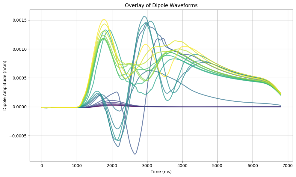
This plot shows an overlay of all smoothed dipole waveforms from the batch simulation. Each line represents a different set of synaptic strength parameters (weight_basket), allowing us to visualize the range of responses across the parameter space. The colormap represents synaptic strengths, from weaker (purple) to stronger (yellow).

As drive strength increases, dipole responses show progressively larger amplitudes and more distinct features, reflecting heightened network activity. Weak drives (purple lines) produce smaller amplitude signals with simpler waveforms, while stronger drives (yellow lines) generate larger responses with more pronounced oscillatory features, indicating more robust network activity.

The y-axis represents dipole amplitude in nAm (nanoAmpere-meters), which is the product of current flow and distance in the neural tissue.

Stronger synaptic connections (yellow lines) generally show larger amplitude responses and more pronounced features throughout the simulation.


        dpl_waveforms, param_values = [], []
for data_list in simulation_results['simulated_data']:
    for data in data_list:
        dpl_smooth = data['dpl'][0].copy().smooth(window_len=30)
        dpl_waveforms.append(dpl_smooth.data['agg'])
        param_values.append(data['param_values']['weight_basket'])

plt.figure(figsize=(10, 6))
cmap = plt.get_cmap('viridis')
log_param_values = np.log10(param_values)
norm = plt.Normalize(log_param_values.min(), log_param_values.max())

for waveform, log_param in zip(dpl_waveforms, log_param_values):
    color = cmap(norm(log_param))
    plt.plot(waveform, color=color, alpha=0.7, linewidth=2)
plt.title('Overlay of Dipole Waveforms')
plt.xlabel('Time (ms)')
plt.ylabel('Dipole Amplitude (nAm)')
plt.grid(True)
plt.tight_layout()
plt.show()

Out:

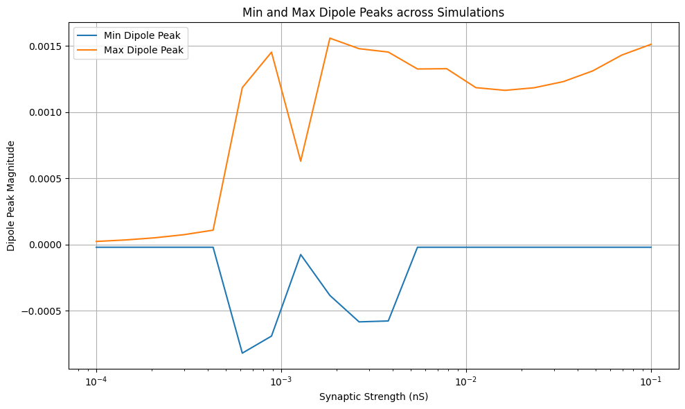
This plot displays the minimum and maximum dipole peaks across different synaptic strengths. This allows us to see how the range of dipole activity changes as we vary the synaptic strength parameter.


        min_peaks, max_peaks, param_values = [], [], []
for summary_list, data_list in zip(simulation_results['summary_statistics'],
                                   simulation_results['simulated_data']):
    for summary, data in zip(summary_list, data_list):
        min_peaks.append(summary['min_peak'])
        max_peaks.append(summary['max_peak'])
        param_values.append(data['param_values']['weight_basket'])

# Plotting
plt.figure(figsize=(10, 6))
plt.plot(param_values, min_peaks, label='Min Dipole Peak')
plt.plot(param_values, max_peaks, label='Max Dipole Peak')
plt.xlabel('Synaptic Strength (nS)')
plt.ylabel('Dipole Peak Magnitude')
plt.title('Min and Max Dipole Peaks across Simulations')
plt.legend()
plt.grid(True)
plt.xscale('log')
plt.tight_layout()
plt.show()

Out: