


7.7: Parallelism: Using the Joblib backend
This example demonstrates how to use the Joblib backend for
simulating dipoles using hnn_core.
hnn_core can take advantage of the Joblib library
to run multiple independent simulations
simultaneously across multiple CPU processors. This is
an example of "embarrassingly
parallel" processing jobs. In HNN, this is commonly done if you want
to run many "trials" of the same simulation. Since each trial simulation
is fully independent of the other trial simulations, each trial
simulation can be run on its own CPU core. Joblib parallelism is
particularly useful if you are using batch
simulation to explore parameter spaces.
Note that Joblib parallelism is distinct from hnn_core's
use of MPI
parallelism, which can be found here.
Authors:
- Mainak Jas ( mjas@mgh.harvard.edu )
- Blake Caldwell ( blake_caldwell@brown.edu )
- Austin Soplata ( austin_soplata@brown.edu )
1. Import Parallel dependencies
Please note that in order to run this tutorial you MUST have installed the "parallel" dependencies for HNN-Core. Normally, these are optional for general HNN-Core use, but they are required for this tutorial. In the next cell, we will check to make sure they are installed, and if they are not, then please follow the directions provided.
                        try:
    import joblib  : F401
except ModuleNotFoundError:
    raise ModuleNotFoundError(
        "\nThe joblib module is required for Joblib parallelism, but it is not "
        "available. Please install the hnn-core package using:\n\n"
        '    pip install "hnn-core[parallel]"\n'
    ) from None
If you installed hnn_core using the Python or Conda
package (i.e. not from source), then you can uncomment and
run the following code cell to easily install the optimization
dependences into your current Python environment. If you do so, please
restart your Jupyter kernel before running the notebook again.
# %pip install -q "hnn-core[parallel]"
After following the above instructions, we should be able to import
JoblibBackend with full parallelism support.
from hnn_core import JoblibBackend
2. Import other dependencies
Let us import what we else need from hnn_core and
matplotlib:
                        import matplotlib.pyplot as plt

from hnn_core import simulate_dipole, neymotin_2020_model
from hnn_core.viz import plot_dipole
3. Setup our network
Following our Alpha example, we will create our network and add a ~10 Hz "bursty" drive:
                        net = neymotin_2020_model()

weights_ampa = {'L2_pyramidal': 5.4e-5, 'L5_pyramidal': 5.4e-5}
net.add_bursty_drive(
    'bursty', tstart=50., burst_rate=10, burst_std=20., numspikes=2,
    spike_isi=10, n_drive_cells=10, location='distal',
    weights_ampa=weights_ampa, event_seed=278)
4. Simulate the trials using JoblibBackend
Finally, we will simulate using the JoblibBackend
class. You can control the number of CPU cores to use via
n_jobs, while the number of total trials to be run can be
specified by n_trials. Note that these numbers do NOT have
to match: you can ask for more trials than there are jobs available, and
Joblib will simply execute later jobs after the first batch has
completed.
                    with JoblibBackend(n_jobs=4):
dpls = simulate_dipole(net, tstop=210., n_trials=6)
5. Visualize the output
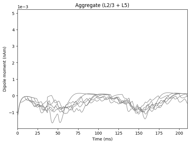
Below, we will see that we have simulated and plotted multiple dipole trials in approximately the time it only takes to do one!
                        plot_dipole(dpls, show=False)
plt.show()