3.1 HNN GUI Quickstart
This tutorial is meant to illustrate the bare minimum usage of the GUI. For more in-depth guidance on using the HNN GUI, see our tutorials in later sections, such as our GUI ERP Tutorial here, GUI Alpha/Beta Tutorial here, or GUI Gamma Tutorial here (also accessible via the sidebar).
Setup
Make sure you have followed our Installation section
here, and are either using HNN in the cloud, using the
conda package, or installing GUI support using
pip.
If you are running HNN “in the cloud”, follow the instructions in the method you have chosen until you can access a webpage that resembles Figure 1.
If you are using a local installation of HNN, then activate your Python environment (see our Local Installation Guide for details), and run the following command in your terminal:
hnn-guiOn Linux, Mac, or native Windows, the above command should open a new tab in your browser which contains the HNN GUI and resembles Figure 1.
Note that if you are on Windows and installed HNN through “Windows
Subsystem for Linux”, then after running the above command, you need to
manually navigate in your browser to the URL that is shown
after[Voila] Voilà is running at:, which is probably http://localhost:8866.
Figure 1

Changing parameters
Click on the tab inside the GUI that says
External drives, then click the box that says
evdist1 (distal). This will expand the box (illustrated in
Figure 2) to show the various parameters that
encompass the external drive to the network called evdist1.
You can use these fields to change parameters of the drive, if you want.
Note that you must scroll down inside the box to see other parameters or
other drives. You can also click the title of the drive again (where it
says evdist1 (distal)) to close the box and see other
drives.
Note that you can always refresh the tab to reset the GUI to its original state: this will clear all parameter changes you have made, but will also delete the GUI data of any simulations you have run in the GUI, unless you previously downloaded the data as a file!
You can also change the parameters of the network itself, as opposed
to the external drives, by clicking on the Network tab and
then clicking on the box of the connection type you want to change,
similar to you accessed the evdist1 drive previously.
Figure 2

Running a simulation
Return to the Simulation tab by clicking the tab. Change
the name of the simulation from default to anything else.
Note that for each new simulation, you must manually change the
name of the simulation, otherwise you will get an error. You can change
the length of time of the simulation using tstop (ms).
Finally, click the purple Run button to run your
simulation! After a minute or two, you should see output resembling Figure 3. This figure shows the 3 external drives
in the top subplot and the total current dipole moment in the
bottom.
Figure 3

Creating more visualizations
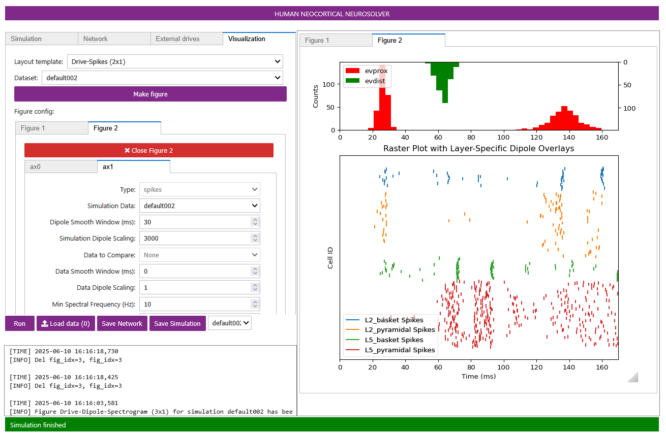
Click the Visualization tab. Then, in the
Layout template drop-down, select
Drive-spikes (2x1). Then, click Make figure.
This will create a new figure on the right, and your screen should
resemble Figure 4. This new figure illustrates
the same drives in the top subplot but a spike rastergram of all
celltypes in the bottom.
Note that for the default simulation, because we are modeling such a
short signal, we cannot generate a spectrogram plot with our default
parameters. If you wish, you can run an additional simulation with a
longer time (a higher tstop value) and then generate an
additional spectrogram plot.
Figure 4
Continue on to other tutorials
Congratulations on running your first simulation, and generating some visualizations of it! We recommend you proceed onto the more detailed GUI ERP Tutorial here, or alternatively the GUI Alpha/Beta Tutorial here or GUI Gamma Tutorial here depending on your scientific interest.