3.2 Optimization in the GUI

This tutorial walks through how to use the Optimization feature of HNN through the GUI. Make sure you have at least gone through 3.1 HNN GUI Quickstart first, so that you understand how to start and use the GUI in general.

For a more in-depth approach that covers similar functionality (and much more), see (Tolley et al., 2026). For tutorials on how to use optimization via the API, see here and here.

1. First simulation

First, let’s load some representative example data that we want to compare a simulation against. Go to our hnn-data repository here (separate from installing HNN) and download this file; on the right side of the page, near where it says Raw, you should see a download symbol. Click that, or feel free to git clone the hnn-data repository as a whole.

1. Start the GUI (see 3.1 HNN GUI Quickstart for how).
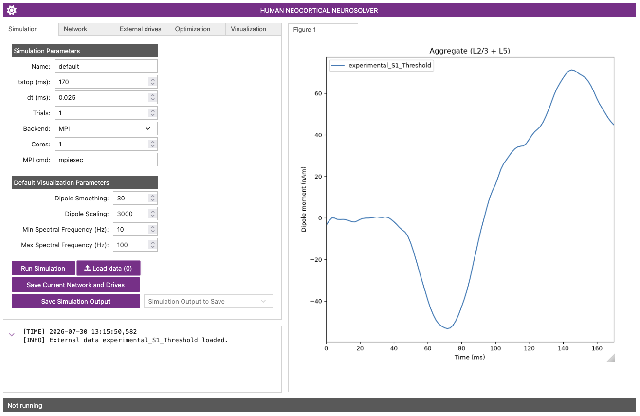
2. Click the Load data button (in the Simulation tab) and load the experimental_S1_Threshold.txt file you just downloaded. A plot showing the data should appear on the right, similar to the figure below:

Figure 1

3. Next to Cores (under Simulation Parameters), increase the number until it increases no further.
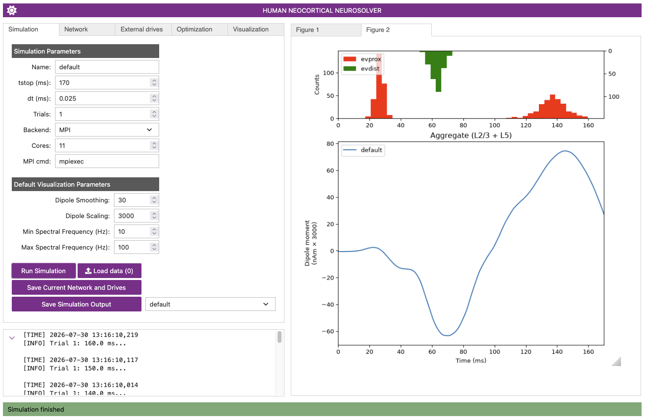
4. Click the Run Simulation button to run the default simulation.
5. Once the simulation has completed, you should see its results on the right, similar to the figure below:

Figure 2

6. Click the Visualization tab.
7. We want to display the simulation versus the experimental data. Click on the entry for Data to Compare, and select the name of the file that you loaded, experimental_S1_Threshold.
8. Next, click the Clear axis button at the bottom (you may have to scroll), and then click Add plot.
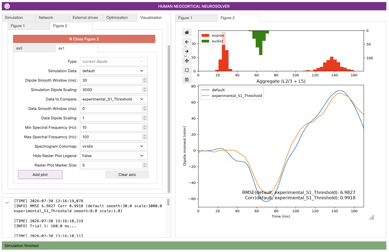
9. You should now see a plot on the right that displays both the simulation (default) and the experimental loaded data, in addition to their root-mean-square-error (around 6.9827) and correlation measures (around 0.9918), similar to this figure:

Figure 3

2. Hand-tuning

Let’s try “hand-tuning” a parameter of one of our drive inputs to see if we can get the simulation to match the experimental data better.

10. Click on the External drives tab.
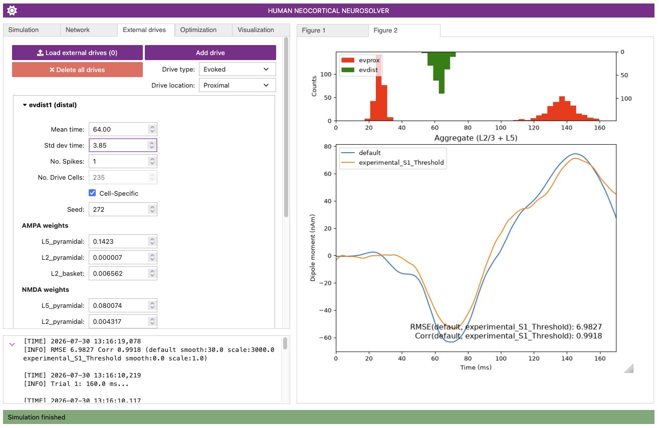
11. Click the box for the first and only distal drive, evdist1.
12. Let’s try changing the mean time of when the distal drive spikes, in the hopes that it will improve how our simulation matches the experiment. Edit the value in the Mean time box to be 64.00. Scientifically, this is analogous to us hypothesizing “What if, in our experiment, the distal input arriving from cortico-cortical and non-lemniscal thalamic sources is arriving slightly later?” Your screen should resemble the following:

Figure 4

13. Click back to the Simulation tab. We are going to run a new simulation.
14. In the Name box, change the simulation name to be something like default-handtune-evdist1 (or whatever you prefer).
15. Click Run Simulation again, after which a new figure will appear on the right.
16. Similar to before, click the Visualization tab, then under Data to Compare, select experimental_S1_Threshold. Next, click the Clear axis button (you may have to scroll down) then the Add plot button. You should see something like the following:

Figure 5

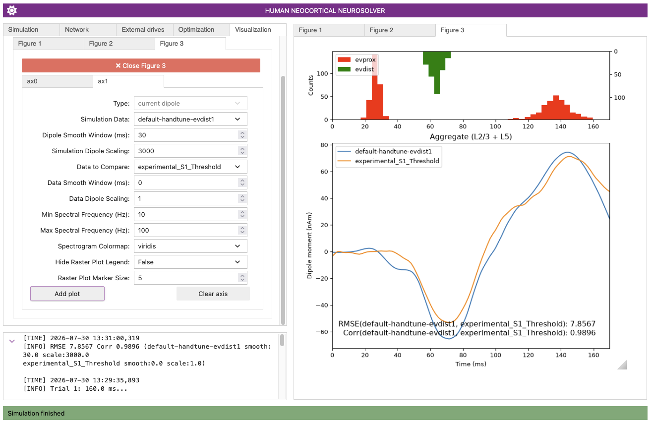
As it turns out, our change made things worse, since now the RMSE has increased to around 7.8567, and our corrrelation has decreased.

3. Optimization

Instead of using manual “hand-tuning” to try to see how changing parameters affects our simulation in relation to some experimental data, we can also use “optimization”. This will run several simulations where one or more parameters have their values changed automatically, and at each step, the computer will run try to get the simulation closer to the “objective” of being similar to the experimental data values. Again, see (Tolley et al., 2026) for more details.

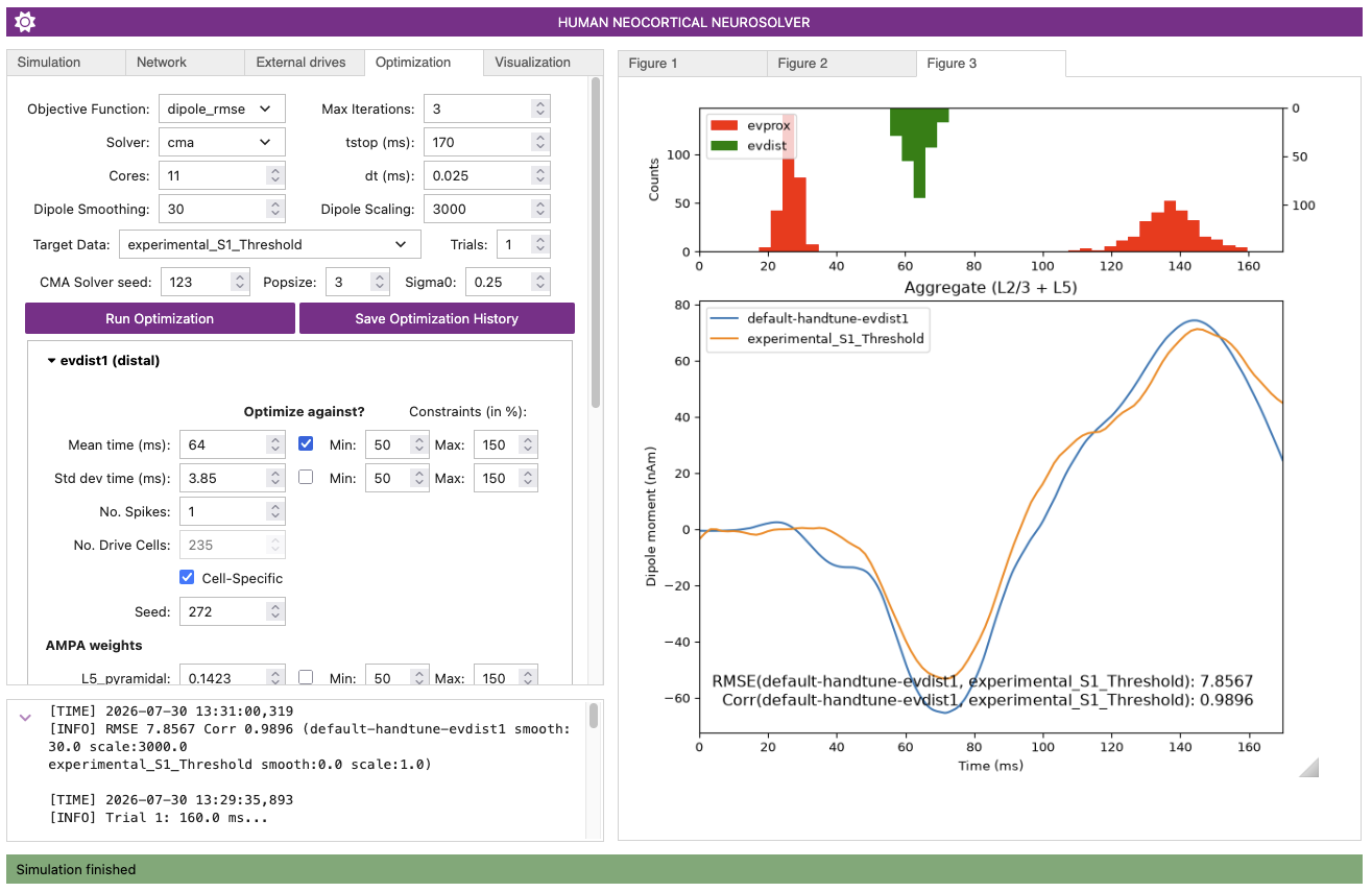
17. Click the Optimization tab.

18. We need to make several changes in this tab:

    1. Decrease Max Iterations to 3.
    2. Change Solver to cma.
    3. For Target Data, select your loaded experimental data (experimental_S1_Threshold)
    4. Click the box for evdist1 to expand it.
    5. Inside the evdist1 box, in the Optimize against? column of checkboxes, check the checkbox for Mean time.
    6. Your GUI should now resemble the following:

Figure 6

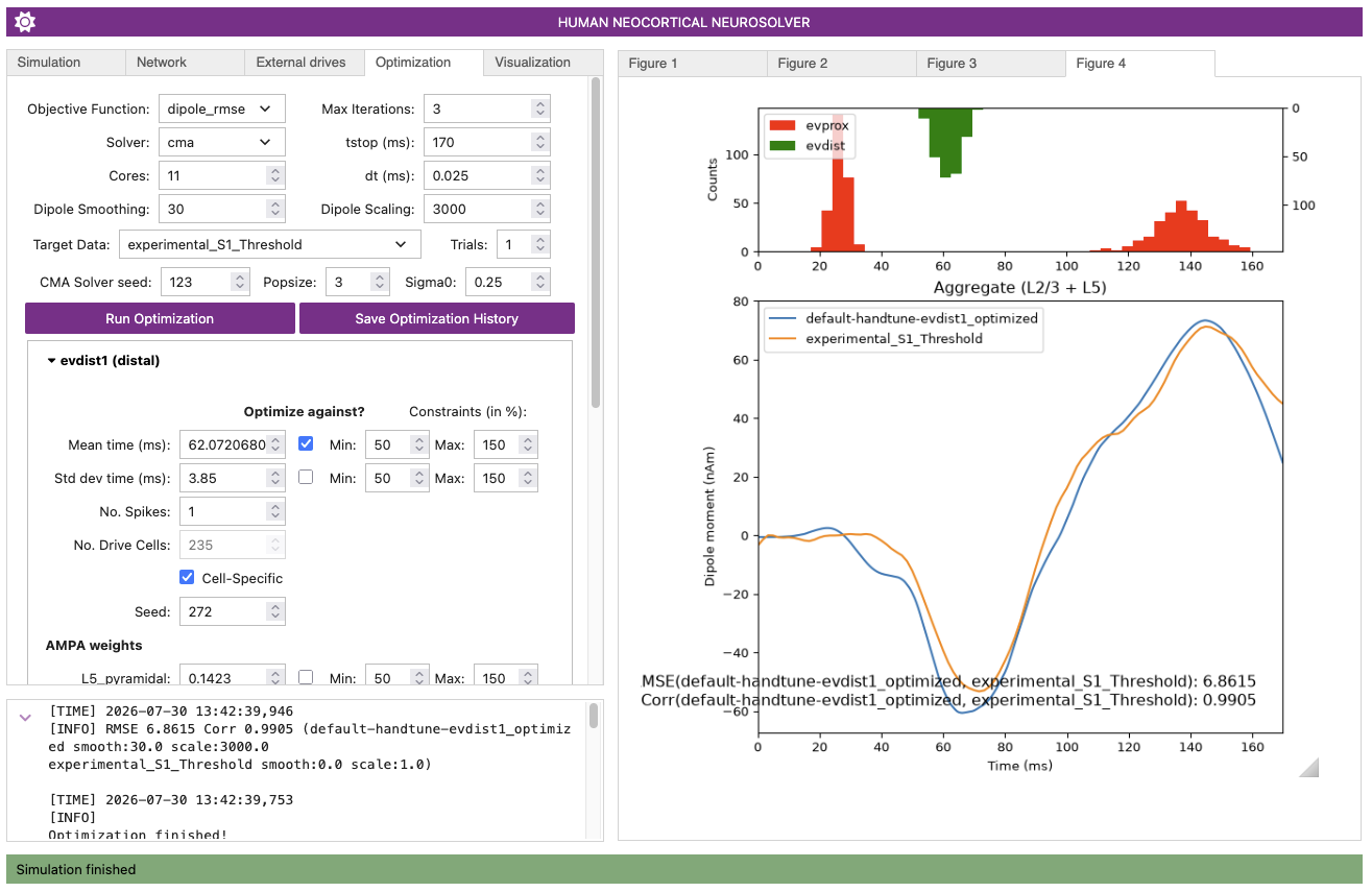
19. Click the Run Optimization tab. Note that depending on your computer speed, this could take up to several minutes.
20. Finally, depending on randomness, you will probably see that the optimization has resulted in an improved fit to your experimental data, in which case the screen will resemble the following:

Figure 7

21. Before we look at the results, click the Save Optimization History button. This will prompt you for where to save a raw text file that includes the history of all the parameters you optimized against, so that you can see what the parameters were both before and after optimization, including their final (optimized) values, and how much they changed.

22. Since we used the default dipole_rmse object, the RMSE value was used during the optimization, and in the example shown above, it has decreased to 6.8615. This is not just a better RMSE value than what we found by hand-tuning (7.8567, viewable by selecting Figure 3 on the right), but in fact slightly better than the default simulation’s as well (6.9827, viewable by selecting Figure 2 on the right).

23. However, note that in our optimized simulation (Figure 4 in the GUI on the right), while some portions of the dipole time series are closer to the experimental data, other portions are farther away from it. This is an important point: a better quantitative fit does not necessarily mean that the scientific validity is better! You must always use your scientific judgment to evaluate if such a parameter change makes sense in the biological system you’re investigating.

24. In HNN, you can optimize against multiple parameters and as many parameters as you want. However, be aware that increasing the number of parameters you optimize against greatly increases the computational cost of the simulations that it needs to run. Additionally, if you want to run many simulations or iterations of the optimization, we strongly recommend that you switch to the API, since the GUI consumes more memory to run simulations than the API.

For tutorials on how to use optimization via the API, see here and here.