
Online HNN Workshop, Spring 2025
Welcome to our Online HNN Workshop for spring 2025! In this interactive workshop, we will begin with a didactic overview of the background and development of HNN. We will then introduce you to the GUI and Python interfaces of HNN through lectures and hands-on investigations of the most commonly measured signals, including ERPs and low-frequency brain rhythms. We will also cover automatic parameter optimization in the Python interface.
Table of Contents
- Workshop Schedule
- Installing and Running HNN
- Downloading Workshop Materials
- ERP Tutorial with HNN GUI
- Simulating Oscillations in the HNN GUI
- Simulating an ERP in the HNN API
- Workshop Feedback
Workshop Schedule
| Morning | ||||
| 9:00 AM - 9:45 AM | Lecture | Overview of HNN with Q&A | Dr. Stephanie Jones | Zoom |
| 10:00 AM - 12:00 PM | Hands-On | Simulating an Event-Related Potential (ERP) in HNN GUI | Dylan Daniels | Zoom |
| 12:00 PM - 1:00 PM | Break | Lunch break and office hours | ||
| Afternoon Path 1: Oscillations in HNN GUI | ||||
| 1:00 PM - 1:20 PM | Lecture | Overview of Oscillations | Dr. Stephanie Jones | Zoom |
| 1:20 PM - 3:00 PM | Hands-On | Simulating oscillations in the HNN GUI | Dr. Austin Soplata | Zoom |
| Afternoon Path 2: ERP and Optimization in the HNN API | ||||
| 1:00 PM - 3:00 PM | Hands-On | Simulating an Event-Related Potential (ERP) in the HNN API | Dr. Carolina Fernandez | Zoom |
Installing and Running HNN
Running HNN GUI in the Cloud (Google CoLab)
We offer many methods to use HNN. To use the HNN GUI without installing it locally, you can use our click here to open our Google CoLab notebook. This is the simplest way to use HNN, but the simulations will take notably longer. This method does require a Google account, but the resources are free and allow you to run HNN GUI at no charge. To run the notebook, click "Runtime" then "Run all", and follow the instructions.
Installing and Running HNN GUI on Your Machine
Click on the section below that matches your operating instructions to view the local installation instructions. If you have any problems installing HNN locally using the instructions below, please use the Google CoLab notebook per the instructions above.
MacOS
If you are new to HNN and biophysical simulations with NEURON, we recommend you do the following to locally install the fastest version of HNN on your Mac computer:
- Download and install the Anaconda Python distribution here, using the default settings.
-
Open a "Terminal" application and install "Xcode Command-Line Tools" by running the following command:
xcode-select --install - Close the Terminal window. If the command says "Command line tools are already installed", move to the next step. If the command takes the time to install itself (approximately 10 minutes), then make sure you restart your computer.
-
After restart, open a new Terminal window. The following commands will remove any existing Conda environments named "hnn-core-env", but it will install HNN with Parallelism/MPI support, which is the fastest version of HNN. Copy, paste, and run the following text:
                        conda activate base

                        conda env remove -y -n hnn-core-env

                        conda create -y -q -n hnn-core-env python=3.12

                        conda activate hnn-core-env

                        mkdir -p $CONDA_PREFIX/etc/conda/activate.d $CONDA_PREFIX/etc/conda/deactivate.d

                        echo "export OLD_DYLD_FALLBACK_LIBRARY_PATH=\$DYLD_FALLBACK_LIBRARY_PATH" >> $CONDA_PREFIX/etc/conda/activate.d/env_vars.sh

                        echo "export DYLD_FALLBACK_LIBRARY_PATH=\$DYLD_FALLBACK_LIBRARY_PATH:\${CONDA_PREFIX}/lib" >> $CONDA_PREFIX/etc/conda/activate.d/env_vars.sh

                        echo "export DYLD_FALLBACK_LIBRARY_PATH=\$OLD_DYLD_FALLBACK_LIBRARY_PATH" >> $CONDA_PREFIX/etc/conda/deactivate.d/env_vars.sh

                        echo "unset OLD_DYLD_FALLBACK_LIBRARY_PATH" >> $CONDA_PREFIX/etc/conda/deactivate.d/env_vars.sh

                        export OLD_DYLD_FALLBACK_LIBRARY_PATH=$DYLD_FALLBACK_LIBRARY_PATH

                        export DYLD_FALLBACK_LIBRARY_PATH=$LD_LIBRARY_PATH:${CONDA_PREFIX}/lib

                        conda install -y -q "openmpi>5" mpi4py -c conda-forge

                        pip install "hnn-core[gui,opt,parallel]"
-
Run the following command, which will print a number to the window. Write down this number somewhere, and later you can enter this number in the "Cores" textbox of the HNN GUI for significant speedup!
                        conda activate hnn-core-env

python -c "import psutil ; print(psutil.cpu_count(logical=False)-1)" -
HNN should now be installed! You should be able to start the GUI by then running the following command in the Terminal window:
                        conda activate hnn-core-env

hnn-gui -
Troubleshooting: If you run into any errors, you may still be able to install HNN locally, but without Parallelism/MPI speedup, by running the following command in the Terminal. If you still cannot run the GUI after running the following command, we recommend you use the Google CoLab method mentioned above. You can also follow our full Installation Guide here and ask us for help with installation after the workshop.
pip install "hnn-core[gui,opt]"
Linux
If you are new to HNN and biophysical simulations with NEURON, we recommend you do the following to locally install the fastest version of HNN on your personal Linux computer. If you have installed NEURON previously, we recommend you uninstall any system-wide package installations of it.
- Download and install the Anaconda Python distribution here, using the default settings.
-
Open a new terminal emulator window. The following commands will remove any existing Conda environments named "hnn-core-env", but it will install HNN with Parallelism/MPI support, which is the fastest version of HNN. Copy, paste, and run the following text:
                        conda activate base

                        conda env remove -y -n hnn-core-env

                        conda create -y -q -n hnn-core-env python=3.12

                        conda activate hnn-core-env

                        mkdir -p $CONDA_PREFIX/etc/conda/activate.d $CONDA_PREFIX/etc/conda/deactivate.d

                        echo "export OLD_LD_LIBRARY_PATH=\$LD_LIBRARY_PATH" >> $CONDA_PREFIX/etc/conda/activate.d/env_vars.sh

                        echo "export LD_LIBRARY_PATH=\$LD_LIBRARY_PATH:\${CONDA_PREFIX}/lib" >> $CONDA_PREFIX/etc/conda/activate.d/env_vars.sh

                        echo "export LD_LIBRARY_PATH=\$OLD_LD_LIBRARY_PATH" >> $CONDA_PREFIX/etc/conda/deactivate.d/env_vars.sh

                        echo "unset OLD_LD_LIBRARY_PATH" >> $CONDA_PREFIX/etc/conda/deactivate.d/env_vars.sh

                        export OLD_LD_LIBRARY_PATH=$LD_LIBRARY_PATH

                        export LD_LIBRARY_PATH=$LD_LIBRARY_PATH:${CONDA_PREFIX}/lib

                        conda install -y -q "openmpi>5" mpi4py -c conda-forge

                        pip install "hnn-core[gui,opt,parallel]"
-
Run the following command, which will print a number to the window. Write down this number somewhere, and later you can enter this number in the "Cores" textbox of the HNN GUI for significant speedup!
                        conda activate hnn-core-env

python -c "import psutil ; print(psutil.cpu_count(logical=False)-1)" -
HNN should now be installed! You should be able to start the GUI by then running the following command in the terminal window:
                        conda activate hnn-core-env

hnn-gui -
Troubleshooting: If you run into any errors, you may still be able to install HNN locally, but without Parallelism/MPI speedup, by running the following command in the terminal. If you still cannot run the GUI after running the following command, we recommend you use the Google CoLab method mentioned above. You can also follow our full Installation Guide here and ask us for help with installation after the workshop.
pip install "hnn-core[gui,opt]"
Windows
If you are using a Windows machine, we strongly recommend you use the Google CoLab method above, since HNN runs slower on Windows, and we currently do not support Parallelism/MPI on Windows. If you still want to install HNN locally on Windows, follow these directions:
- Download and install the Anaconda Python distribution here, using the default settings.
- Download and install the Windows-specific NEURON binaries here, using the default settings.
- Open the application "Anaconda Navigator" and create a new Python environment with Python version 3.12 or below.
-
Open a Terminal in the new Python environment and run the following command:
pip install "hnn-core[gui,opt]" -
HNN should now be installed! You should be able to start the GUI by then running the following command in the terminal window:
hnn-gui - Troubleshooting: If you run into any errors, then please use the Google CoLab method above.
Downloading Workshop Materials
To follow along with the interactive portions of the workshop, you will need to download the workshop materials available in the workshop materials folder of our hnn-data GitHub repository.
To only retrieve the required materials for the hands-on ERP Tutorial with HNN GUI, you can click here to download the necessary files from Download Directory.
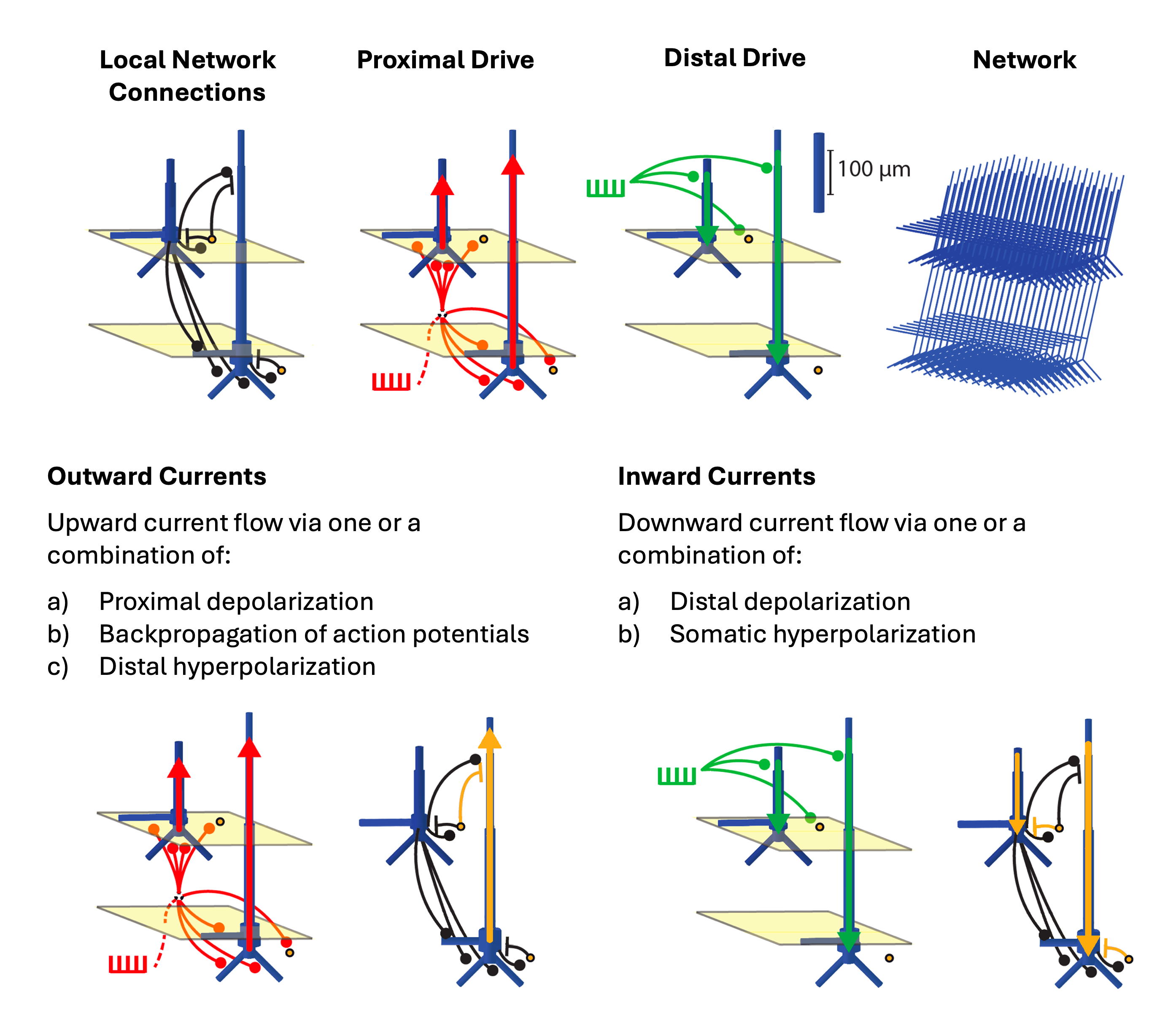
Additionally, we will refer to the schematic below throughout the workshop, and we include it here for your reference.
Figure A
ERP Tutorial with HNN GUI
In this section of the hands-on workshop, we will walk through the steps for 1) simulating an ERP in the GUI, and 2) adjusting model parameters to get a better match to experimental data.
The primary goal of this segment of the workshop is to give you an example of how to use HNN to explore the neural mechanisms underlying the recorded signals in your own experimental data.
Specifically, we provide you with source-localized MEG data from a tactile detection task (see our ERP tutorial for more information on the data and the experimental design), and we walk you through the process of 'hand-tuning' the timing and strengths of the external drives to the network.
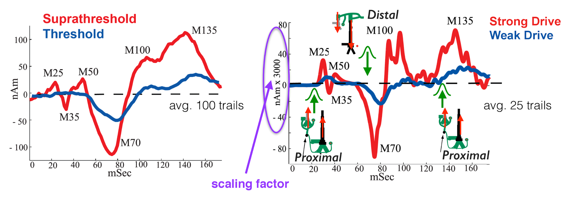
Below, we include a figure from our lab's published work (see Jones et al., 2007) that shows the experimental data we will be using in this tutorial (left panel), as well as the simulated evoked responses used in the paper (right panel). We will reference this figure in the sections that follow.
Figure B
For each exercise in the GUI walkthrough, we will provide a set of steps you can follow to reach the intended 'starting point' for completing the exercise. (The 'starting point' is the assumed state of the GUI before you begin the exercise.)
Interactive Exercise 1
In this exercise, we will adjust the Smooth Window and the Dipole Scaling of the simulated waveform to see if we can get a better match to the experimental data we load into HNN.
Remember that "scaling" in this case refers to a scaling factor applied to our simulated waveform. You can think of the scaling factor as a measure of the number of cells contributing to the simulated signal. "Smoothing" is also related to the number of cells contributing to the signal, and can be thought of as the effect of averaging across a large population of cells.
Exercise 1 Starting Point
- Refresh the HNN GUI to restore the default state.
-
Click
Load data. -
From the "workshops/erp_gui_walkthrough" directory of the "hnn-data" folder, select the
experimental_S1_SupraT.txtdata file. -
Click
Runto run the "default" simulation -
Click the
Visualizationtab. This should bring you to the tab "ax1" of "Figure 2", corresponding to the lower subplot of Figure 2. -
Under the "ax1" tab, click on the downdown box next to
Data to compareand selectexperimental_S1_SupraT. -
Click the
Clear axisbutton at the bottom of the "ax1" tab -
Click the
Add plotbutton
Exercise 1.1
-
From the
Visualizationtab, adjust theDipole Smooth Window (ms)in the dipole plot produced by your simulation. - If you're following from the Exercise 1 Starting Point outlined above, this would correspond to the "ax1" tab of "Figure 2".
- Note that "ax1" in this case refers to the lower subplot of Figure 2 and has a "Type" of "current dipole"
-
If you need to plot the data, ensure that
Data to compareis set toexperimental_S1_SupraT. Otherwise, set it toNone. -
Try each of the following values:
-
Value 1: 0 -
Value 2: 15 -
Value 3: 90
-
-
After each update to the value of
Dipole Smooth Window, clickAdd plotto overlay the new dipole on your figure. -
Alternatively, you can first click
Clear axisand thenAdd plotif you do not want to overlay your new dipole on the same plot.
Note that you do not need to re-run the simulation when changing parameters in the Visualization tab.
|
Discussion Questions:
- What is the effect of increasing the smoothing window on the waveform shape?
- How do you determine the "right" level of smoothing?
Exercise 1.2
-
Reset the
Dipole Smooth Window (ms)to its default value of30 -
Click
Clear axis -
Ensure the
Simulation Datafield is set todefault, and theData to Comparefield is set toexperimental_S1_SupraT -
Next, click
Add plot. This should reset your figure to the state it was in before Exercise 1.1. -
Set the
Data to Comparefield toNone -
Next, adjust the
Simulation Dipole Scalingin your figure. -
Try each of the following values:
-
Value 1: 1500 -
Value 2: 5000 -
Value 3: 10000
-
-
After each update to the value of
Simulation Dipole Scaling, clickAdd plotto overlay the new dipole on your figure.
Discussion Questions:
- How does changing the scaling factor affect the waveform shape?
- Why might you choose one scaling value over another?
Exercise 1.3
Let's now load a different set of evoked drives that was tuned for the suprathreshold experimental condition and compare the new simulation to the default simulation.
-
Select the
External Drivestab -
Click the
Load external drivesbutton. -
From the "workshops/erp_gui_walkthrough" directory of the "hnn-data" folder, select the
ERPSupraT_All_Drives.jsonparameter file. -
In the
Simulationtab, change the name of the simulation toAll_Drives -
Click
Runto start the simulation -
Once your simulation has finished, navigate to the
Visualizationtab. -
From your newly-generated figure, click on the
Data to comparedropdown box and selectexperimental_S1_SupraT -
Click
Clear axisand thenAdd plot
Discussion Questions:
- What differences do you observe in the input histograms and the dipole waveforms for the two simulations?
- Which simulation yields a lower RMSE when compared to the data? Which simulation yields a dipole that more closely matches the shape of the experimental data?
- Is it the case that the simulation with the lower RMSE is always the better starting point when "tuning" the simulation to experimental data? Why might you choose one simulation over another as a starting point?
| Note that you can use any of the network configuration we provide in 'hnn-data' as a starting point when "tuning" your simulations to your experimental data. |
Interactive Exercise 2
In this exercise, we will focus on hand tuning the parameters for the first proximal drive only. The goal is to improve the fit of the simulated waveform to the experimental data, focusing solely on the first peak (referred to as the "M25" peak in our published work and in Figure B above).
Exercise 2 Starting Point
- If needed, refresh the page to return the HNN GUI to the default state. Note that previous simulations will be cleared when refreshing the page.
-
Click
Load data -
From the "workshops/erp_gui_walkthrough" directory of the "hnn-data" folder, select the
experimental_S1_SupraT.txtdata file. -
Click
Runto run the "default" simulation. -
From the
External drivestab, click theLoad external drivesbutton and select the select theERPSupraT_All_Drives.jsonparameter file from the "workshops/erp_gui_walkthrough" directory of the "hnn-data" folder. -
In the
Simulationtab, change the name of the simulation toAll_Drives -
Click
Runto run the "All_Drives" simulation.
Exercise 2.1
In this exercise, we'll be adjusting the AMPA weights for the first proximal drive to the Layer 2/3 and Layer 5 pyramidal neurons, and we'll explore how changing these variables affects our simulation.
Since we'll be looking at the first proximal drive only, as noted above, we'll first need to remove the other drives and re-run the simulation.
-
From the
External Drivestab, delete the drives labelledevdist1andevprox2. -
You can do so by selecting the drive and then clicking the
Deletebutton at the bottom of the drive parameters. -
Alternatively, you can click the
Load external drivesbutton and load theERPSupraT_Prox1.jsonparameter file from "hnn-data" -
From the
Simulationtab, change the "Name" field toProx1_Only -
Click the
Runbutton to run the "Prox1_Only" simulation. -
From the
Visualizationtab, overlay the experimental data on your newly-generated figure by settingData to comparetoexperimental_S1_SupraT -
Click
Clear axisand thenAdd plot
One you've added the data to your figure, select the drive labelled evprox1 from the list of drives in the External drives tab. You should now see all of the editable drive parameters for the first proximal drive.
Next, adjust the values of the Layer 2/3 (L2) and Layer 5 (L5) pyramidal cell AMPA weights. Try the following combinations:
-
Simulation 01:
-
Name (suggested): Prox1_Only_01 -
L5_pyramidal AMPA weight ("evprox1"): 0.2400 -
L2_pyramidal AMPA weight ("evprox1"): 1.0515
-
-
Simulation 02:
-
Name (suggested): Prox1_Only_02 -
L5_pyramidal AMPA weight ("evprox1"): 0.0480 -
L2_pyramidal AMPA weight ("evprox1"): 0.2103
-
Once you've run the two simulations above, create a new Figure that displays all of the simulated dipoles and the experimental data on the same graph.
You can do this by selecting any previously-generated figure and adding your new simulations to the dipole plot. For example, if you're working from the Starting Point outlined above:
-
Select "ax1" of "Figure 2" from the
Visualizationtab -
Click the
Simulation Datadropdown and select one of your new simulations. -
If you need to plot the data, ensure that
Data to compareis set toexperimental_S1_SupraT. Otherwise, set it toNone. -
Click the
Add plotbutton. - Repeat these steps for each simulation you would like to compare.
Discussion Questions:
- How do the AMPA weights relate to current flow in our simulation? Refer to Figure A above for a visual representation of the network and drives.
- Which of these three simulations is the "best"? You should choose your "best" simulation based on which one most closely matches the "M25" peak, as shown in Figure B above.
Exercise 2.2
Next, compare and contrast the dipoles and the spiking profiles for the initial simulation (before changing the AMPA weights) and your "best" simulation (after changing the AMPA weights).
You can create a raster plot with the layer-specific dipoles overlaid by following the steps below:
-
Select
Dipole Layers-Spikes (1x1)from the "Layout template" dropdown menu in theVisualizationtab. -
Doing so will trigger the
Datasetdropdown box to appear below the "Layout template" dropdown. -
From the "Dataset" dropdown box, select your simulation and then click
Make figure. - Repeat these steps for each simulation you want to visualize
Discussion Questions:
- What differences do you observe in the layer-specific dipoles and the spiking profiles between the initial simulation and the "best" simulation?
-
Try changing the
Dipole Smooth Windowto0, and then regenerate the spiking profile. Does this change your interpretation of how the spiking relates to the layer-specific dipoles?
Exercise 2.3
Next, we'll "turn off" the driving inputs to the Layer 2/3 and Layer 5 basket cells by setting their weights to 0, and we'll see how that changes our results. Before running the simulation, take a moment to consider what you think will happen to the dipole and to the spiking.
-
From the
External Drivestab, first set the AMPA weights for the Layer 2/3 and Layer 5 pyramidal neurons to the values from Exercise 2.1 that produced the "best" fit to the "M25" peak. -
Next, set the AMPA and NMDA weights to
0for theL5_basketandL2_basketcells in theevprox1drive parameters. -
From the
Simulationtab, change the value of the "Name" field toProx1_Only_noBasket -
Click
Runto run the "Prox1_Only_noBasket" simulation.
You can create a raster plot with the layer-specific dipoles overlaid by following the steps in Exercise 2.2 above.
Discussion Questions:
-
What happens to the dipole when you set the basket cell AMPA/NMDA weights to
0? - What changes do you observe in the spiking profile, and what might be driving those changes?
Interactive Exercise 3
In this section, we will hand tune the parameters for the first distal drive. The goal is to improve the fit of the simulated waveform to the experimental data, focusing on the trough at ~ 70ms ("M70").
Exercise 3 Starting Point
-
Follow all instructions in the
Exercise 2 Starting Pointsection above -
From the
External drivestab, click theLoad external drivesbutton and select the select theERPSupraT_Prox1.jsonparameter file from the "workshops/erp_gui_walkthrough" directory of the "hnn-data" folder. -
From the
Simulationtab, change the "Name" field toProx1_Only -
Click the
Runbutton to run the "Prox1_Only" simulation.
Exercise 3.1
In this exercise, we'll be adjusting the timing of the first distal drive, and we'll explore how doing so affects our simulation.
This time, we'll start by load in a parameter set that includes the "tuned" version of the first proximal drive, as well as the un-tuned distal drive.
-
Select the
External Drivestab. -
Click the
Load external drivesbutton. From the "workshops/erp_gui_walkthrough" directory of the "hnn-data" folder, select theSupraT_Prox1_Dist1.jsonparameter file. -
From the
Simulationtab, change the value of the "Name" field toP1_D1 -
Click
Runto run the "P1_D1" simulation. -
From the
Visualizationtab, overlay the experimental data on your newly-generated figure by settingData to comparetoexperimental_S1_SupraT -
Click
Clear axisand thenAdd plot
Next, we'll try adjusting the standard deviation of the distal drive. Note that this is only one parameter that affects the timing of the driving input.
Before running the simulations below, take a moment to consider what you think will happen to the dipole and to the spiking.
-
From the
External Drivestab, selectevdist1. You should now see all of the editable drive parameters for the distal drive. -
Adjust the value of the standard deviation around the mean arrival time, listed as:
Std dev time. - Try the following combinations:
-
Simulation 01:
-
Name (suggested): P1_D1_01 -
Std dev time: 13.81
-
-
Simulation 02:
-
Name (suggested): P1_D1_02 -
Std dev time: 3.81
-
Compare the layer-specific dipoles and the spiking profiles for each simulation, as done in Exercise 2.2 above.
Discussion Questions:
- How does increasing / decreasing the standard deviation of the distal drive's arrival time affect the amplitude of the "M70" trough"?
- What differences do you observe in the raster plots for the different simulations? How do the differences in spiking relate to the differences observed in the layer-specific dipoles?
Interactive Exercise 4
In this section, we will hand tune the parameters for the second proximal drive, with the goal of continuing to improve the fit of the simulated waveform to the experimental data.
Note that we will simulate a single peak that fits the overall shape of both the "M100" and "M135" peaks shown in Figure B. Capturing the nuanced dynamics that yield the two distinct "M100" and "M135" peaks requires simulating many trials, as we do in our published work. So we simplify the exercise here for illustrative purposes and to make it feasible to run the exercises in a short amount of time.
Exercise 4 Starting Point
-
Follow all instructions in the
Exercise 2 Starting PointandExercise 3 Starting Pointsections above -
From the
External drivestab, click theLoad external drivesbutton and select the select theERPSupraT_Prox1_Dist1.jsonparameter file from the "workshops/erp_gui_walkthrough" directory of the "hnn-data" folder. -
From the
Simulationtab, change the "Name" field toP1_D1 -
Click the
Runbutton to run the "P1_D1" simulation.
Exercise 4.1
In this exercise, we'll be adjusting the timing of the second proximal drive, and we'll explore how doing so affects our simulation.
This time, we'll start by load in a parameter set that includes the "tuned" version of the first proximal and first distal drives, as well as the "un-tuned" second proximal drive.
-
Select the
External Drivestab. -
Click the
Load external drivesbutton. From the "workshops/erp_gui_walkthrough" directory of the "hnn-data" folder, select theSupraT_Prox1_Dist1_Prox2.jsonparameter file. -
From the
Simulationtab, change the value of the "Name" field toP1D1P2 -
Click
Runto run the "P1D1P2" simulation. -
From the
Visualizationtab, overlay the experimental data on your newly-generated figure by settingData to comparetoexperimental_S1_SupraT -
Click
Clear axisand thenAdd plot
Next, we'll try adjusting the mean arrival time of the second proximal drive, which is another parameter (in addition to the standard deviation) that affects the timing of the driving inputs.
Before running the simulations below, take a moment to consider what you think will happen to the dipole and to the spiking.
-
From the
External Drivestab, selectevprox2. You should now see all of the editable drive parameters for the second proximal drive. -
Adjust the value of the mean arrival time of the drive, listed as:
Mean time. - Try the following combinations:
-
Simulation 01:
-
Name (suggested): P1D1P2_01 -
Mean time: 105
-
-
Simulation 02:
-
Name (suggested): P1D1P2_02 -
Std dev time: 95
-
Compare the layer-specific dipoles and the spiking profiles for each simulation, as done in Exercise 2.2 above.
Discussion Questions:
- How does changing the mean arrival time of the second proximal drive affect the amplitude of the "M135" peak? Explain your reasoning.
- Does changing the mean arrival time of the second proximal drive affect other parts of the dipole? If so, what difference do you observe in other time windows, and why might this be the case?
Interactive Exercise 5
Now that you have simulated all three drives, you may notice that there are still some discrepancies between the simulated data and the experimental data. What additional parameters might you adjust to continue to improve the fit? Try to adjust the timing and strength of any of the external drives and see if you can get a RMSE value less than 18.5.
Note that some features of the waveform will be difficult to capture when we're only simulating one trial due to the lack of stochasticity. In practice, we would simulate a large number of trials and tune to the average waveform. However, there is still room for improvement even when simulating only one trial.
Discussion Questions:- Which parameters did you change and why?
- Did your parameter changes always yield the results you expected? If not, can you explain the discrepancies? (Hint: try looking at the spiking plots and the layer-specific dipoles in conjunction with the schematic above.)
Once you've run some simulations and answered the above questions, you can load our "solution" from the External Drives tab by clicking the Load external drives button and selecting the "ERPSupraT_hand-tuned.json" file from the "workshops/erp_gui_walkthrough" directory of the "hnn-data" folder. Note that our "solution" is merely one possible answer among many, and so don't feel constrained by the solution we provide.
Simulating Oscillations in the HNN GUI
In this section, we will be simulating oscillations in the HNN GUI.
Click here to join the hand-on session with Dr. Soplata.
To follow along with the interactive portions of the workshop, please click here to be redirected to the Alpha-Beta GUI tutorial.
Simulating an Event-Related Potential (ERP) in the HNN API
In this section, we will cover how to simulation an ERP in the HNN API, and we will also cover how to use HNN's built-in optimization features. To follow along with Dr. Fernandez, please access the CoLab notebooks via the following links:
- Simulating ERPs with HNN API
- Note that this notebook largely empty, as Dr. Fernandez will be "live coding" for this portion of the workshop.
- We will send out the "filled in" version of this notebook at the end of the session
- Optimizing ERPs with HNN API
Workshop Feedback
Thank you for attending our workshop! We would very much appreciate it if you took a few minutes to complete our Workshop Feedback survey. This information is used for reporting purposes for the grants that fund our continued development, and it also helps us improve our software to make it more useful for our users. Survey results are also completely anonymous, as we do not collect name or email.