4.3: Modifying local connectivity
This example demonstrates how to modify the network connectivity.
        # Author: Nick Tolley

import os.path as op

import matplotlib.pyplot as plt
Let us import hnn_core.
        import hnn_core
from hnn_core import jones_2009_model, simulate_dipole
To explore how to modify network connectivity, we will start with
simulating the evoked response from the ERP
example and explore how it changes with new connections. We first
instantiate the network. (Note: Setting
add_drives_from_params=True loads a set of predefined
drives without the drives API shown previously).
net_erp = jones_2009_model(add_drives_from_params=True)
Instantiating the network comes with a predefined set of connections
that reflect the canonical neocortical microcircuit.
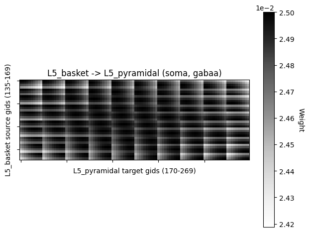
net.connectivity is a list of dictionaries which detail
every cell-cell, and drive-cell connection. The weights of these
connections can be visualized with hnn_core.viz.plot_connectivity_matrix
as well as hnn_core.viz.plot_cell_connectivity.
We can search for specific connections using
pick_connection which returns the indices of
net.connectivity that match the provided parameters.
from hnn_core.viz import plot_connectivity_matrix, plot_cell_connectivity, plot_drive_strength
from hnn_core.network import pick_connection
print(len(net_erp.connectivity))
conn_indices = pick_connection(
net=net_erp, src_gids='L5_basket', target_gids='L5_pyramidal',
loc='soma', receptor='gabaa')
conn_idx = conn_indices[0]
print(net_erp.connectivity[conn_idx])
plot_connectivity_matrix(net_erp, conn_idx, show=False)
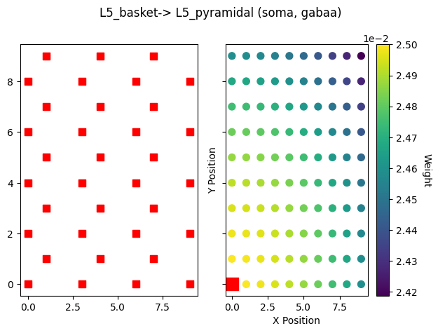
# Note here that `'src_gids'` is a `set` object
# The `.pop()` method can be used to sample a random element
src_gid = net_erp.connectivity[conn_idx]['src_gids'].copy().pop()
fig = plot_cell_connectivity(net_erp, conn_idx, src_gid, show=False)
plt.show()
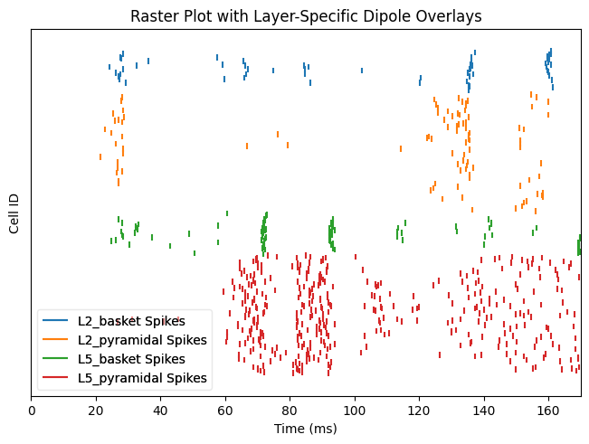
Data recorded during simulations are stored under CellResponse. Spiking activity can be visualized after a simulation is using CellResponse.plot_spikes_raster:
        dpl_erp = simulate_dipole(net_erp, tstop=170., n_trials=1)
net_erp.cell_response.plot_spikes_raster(show=False)
plt.show()
We can also define our own connections to test the effect of
different connectivity patterns. To start,
net.clear_connectivity() can be used to clear all
cell-to-cell connections. By default, previously defined drives to the
network are retained, but can be removed with
net.clear_drives(). net.add_connection is then
used to create a custom network. Let us first create an all-to-all
connectivity pattern between the L5 pyramidal cells, and L2 basket
cells. Network.add_connection
allows connections to be specified with either cell names, or the cell
IDs (gids) directly.
        def get_network(probability=1.0):
    net = jones_2009_model(add_drives_from_params=True)
    net.clear_connectivity()

    # Pyramidal cell connections
    location, receptor = 'distal', 'ampa'
    weight, delay, lamtha = 1.0, 1.0, 70
    src = 'L5_pyramidal'
    conn_seed = 3
    for target in ['L5_pyramidal', 'L2_basket']:
        net.add_connection(src, target, location, receptor,
                           delay, weight, lamtha, probability=probability,
                           conn_seed=conn_seed)

    # Basket cell connections
    location, receptor = 'soma', 'gabaa'
    weight, delay, lamtha = 1.0, 1.0, 70
    src = 'L2_basket'
    for target in ['L5_pyramidal', 'L2_basket']:
        net.add_connection(src, target, location, receptor,
                           delay, weight, lamtha, probability=probability,
                           conn_seed=conn_seed)
    return net


net_all = get_network()
dpl_all = simulate_dipole(net_all, tstop=170., n_trials=1)
We can additionally use the probability argument to
create a sparse connectivity pattern instead of all-to-all. Let's try
creating the same network with a 10% chance of cells connecting to each
other.
        net_sparse = get_network(probability=0.1)
dpl_sparse = simulate_dipole(net_sparse, tstop=170., n_trials=1)
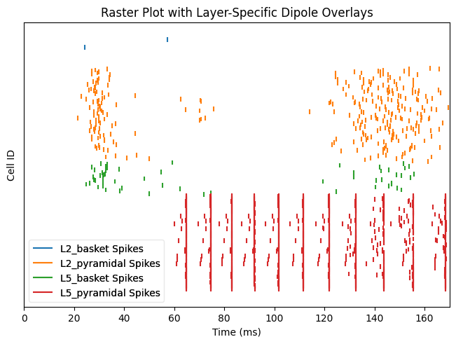
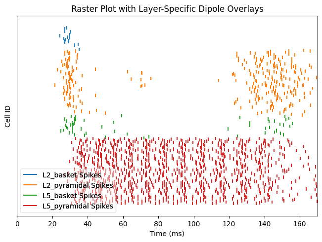
With the previous connection pattern there appears to be synchronous rhythmic firing of the L5 pyramidal cells with a period of 10 ms. The synchronous activity is visible as vertical lines where several cells fire simultaneously Using the sparse connectivity pattern produced a lot more spiking in the L5 pyramidal cells.
        net_all.cell_response.plot_spikes_raster(show=False)
net_sparse.cell_response.plot_spikes_raster(show=False)
plt.show()
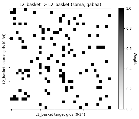
We can plot the sparse connectivity pattern between cell populations.
        conn_indices = pick_connection(
    net=net_sparse, src_gids='L2_basket', target_gids='L2_basket',
    loc='soma', receptor='gabaa')

conn_idx = conn_indices[0]
plot_connectivity_matrix(net_sparse, conn_idx, show=False)
plt.show()
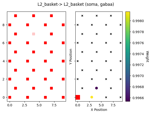
Note that the sparsity is in addition to the weight decay with distance from the source cell.
        src_gid = net_sparse.connectivity[conn_idx]['src_gids'].copy().pop()
plot_cell_connectivity(net_sparse, conn_idx, src_gid=src_gid, show=False)
plt.show()
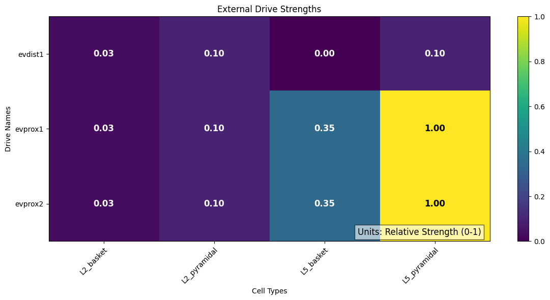
We can plot the strengths of each external drive across each cell types.
# This can be done in a relative way, enabling you to compare the proportion
# coming from each drive:
plot_drive_strength(net_erp, show=False)
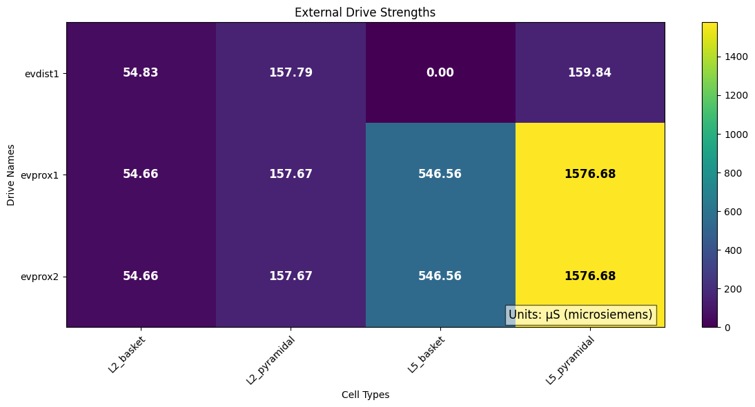
# Alternatively, you can compare the total amount of each drive in conductance:
plot_drive_strength(net_erp, normalize=False, show=False)
plt.show()
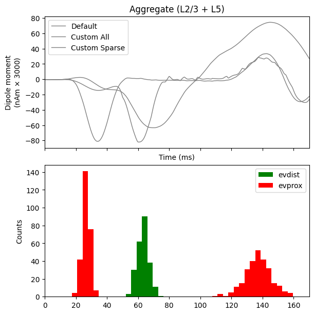
In the sparse network, there still appears to be some rhythmicity where the cells are firing synchronously with a smaller period of 4-5 ms. As a final step, we can see how this change in spiking activity impacts the aggregate current dipole.
        from hnn_core.viz import plot_dipole
fig, axes = plt.subplots(2, 1, sharex=True, figsize=(6, 6),
                         constrained_layout=True)

window_len = 30  # ms
scaling_factor = 3000
dpls = [dpl_erp[0].smooth(window_len).scale(scaling_factor),
        dpl_all[0].smooth(window_len).scale(scaling_factor),
        dpl_sparse[0].smooth(window_len).scale(scaling_factor)]

plot_dipole(dpls, ax=axes[0], layer='agg', show=False)
axes[0].legend(['Default', 'Custom All', 'Custom Sparse'])
net_erp.cell_response.plot_spikes_hist(
    ax=axes[1], spike_types=['evprox', 'evdist'], show=False)
plt.show()