4.4: Animating HNN simulations
This example demonstrates how to animate HNN simulations
# Author: Nick Tolley
First, we'll import the necessary modules for instantiating a network and running a simulation that we would like to animate.
        import os.path as op

import matplotlib.pyplot as plt

import hnn_core
from hnn_core import jones_2009_model, simulate_dipole, read_params
from hnn_core.network_models import add_erp_drives_to_jones_model
We begin by instantiating the network. For this example, we will reduce the number of cells in the network to speed up the simulations.
        net = jones_2009_model(mesh_shape=(3, 3))

# Note that we move the cells further apart to allow better visualization of
# the network (default inplane_distance=1.0 µm).
net.set_cell_positions(inplane_distance=300)
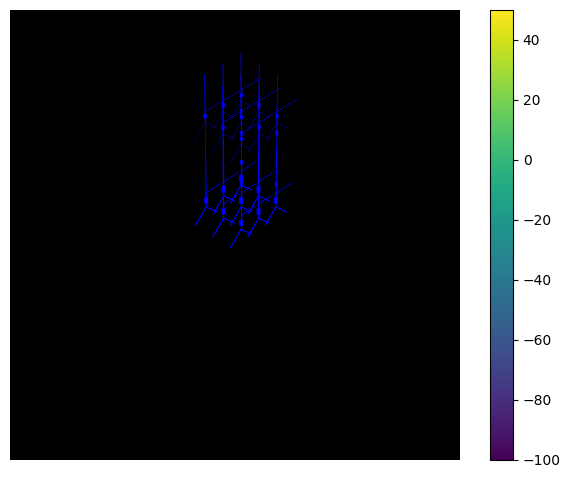
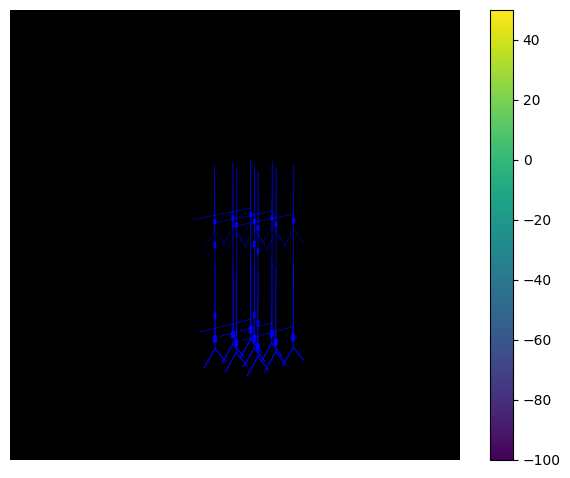
The NetworkPlotter class can be used to visualize the 3D structure of the network.
        from hnn_core.viz import NetworkPlotter

net_plot = NetworkPlotter(net)

We can also visualize the network from another angle by adjusting the azimuth and elevation parameters.
        net_plot.azim = 45
net_plot.elev = 40
net_plot.fig
Next we add event related potential (ERP) producing drives to the
network and run the simulation (see the ERP
simulation for more details). To visualize the membrane potential of
cells in the network, we need to pass
record_vsec='all' to
simulate_dipole(...), which turns on the recording of
voltages in all sections of all cells in the network.
        add_erp_drives_to_jones_model(net)
dpl = simulate_dipole(net, tstop=170, record_vsec='all')
net_plot = NetworkPlotter(net)  # Reinitialize plotter with simulated network
Finally, we can animate the simulation using the
export_movie() method. We can adjust the xyz limits of the
plot to better visualize the network.
        # # If you want to save the animation to a file, then uncomment the code in this cell.
# net_plot.xlim = (400, 1600)
# net_plot.ylim = (400, 1600)
# net_plot.zlim = (-500, 1600)
# net_plot.azim = 225
# net_plot.export_movie('animation_demo.gif', dpi=100, fps=30, interval=100)