03. Simulate gamma rhythms

This example demonstrates how to simulate gamma rhythms generated by the “PING” mechanism using hnn-core 1, 2. Note that the parameter file used is different from other examples: the intrinsic connectivity of the network was tuned in 1 by adjusting the synaptic weights between excitatory (pyramidal) and inbitory (basket) cells until gamma rhythms could be observed. The network dynamics are driven by Poisson-distributed (noisy) spike trains to layer II/III and layer V pyramidal cell populations.

# Authors: Mainak Jas <mainak.jas@telecom-paristech.fr>
#          Sam Neymotin <samnemo@gmail.com>
#          Christopher Bailey <bailey.cj@gmail.com>

# sphinx_gallery_thumbnail_number = 2

import os.path as op

Let us import hnn_core

import hnn_core
from hnn_core import simulate_dipole, read_params, Network

hnn_core_root = op.dirname(hnn_core.__file__)

Read the parameter file and print the between-cell connectivity parameters. Note that these are different compared with the ‘default’ parameter set used in, e.g., 02. Simulate alpha and beta waves.

params_fname = op.join(hnn_core_root, 'param', 'gamma_L5weak_L2weak.json')
params = read_params(params_fname)
print(params['gbar_L*'])

Out:

{
    "gbar_L2Basket_L2Basket": 0.01,
    "gbar_L2Basket_L2Pyr_gabaa": 0.007,
    "gbar_L2Basket_L2Pyr_gabab": 0.0,
    "gbar_L2Basket_L5Pyr": 0.0,
    "gbar_L2Pyr_L2Basket": 0.0012,
    "gbar_L2Pyr_L2Pyr_ampa": 0.0,
    "gbar_L2Pyr_L2Pyr_nmda": 0.0,
    "gbar_L2Pyr_L5Basket": 0.0,
    "gbar_L2Pyr_L5Pyr": 0.0,
    "gbar_L5Basket_L5Basket": 0.0075,
    "gbar_L5Basket_L5Pyr_gabaa": 0.08,
    "gbar_L5Basket_L5Pyr_gabab": 0.0,
    "gbar_L5Pyr_L5Basket": 0.00091,
    "gbar_L5Pyr_L5Pyr_ampa": 0.0,
    "gbar_L5Pyr_L5Pyr_nmda": 0.0
}

We’ll add a tonic Poisson-distributed excitation to pyramidal cells and simulate the dipole moment in a single trial (the default value used by simulate_dipole is n_trials=params['N_trials']).

net = Network(params)

weights_ampa = {'L2_pyramidal': 0.0008, 'L5_pyramidal': 0.0075}
synaptic_delays = {'L2_pyramidal': 0.1, 'L5_pyramidal': 1.0}
rate_constant = {'L2_pyramidal': 140.0, 'L5_pyramidal': 40.0}
net.add_poisson_drive(
    'poisson', rate_constant=rate_constant, weights_ampa=weights_ampa,
    location='proximal', synaptic_delays=synaptic_delays, seedcore=1079)

dpls = simulate_dipole(net)

Out:

joblib will run over 1 jobs
Building the NEURON model
[Done]
running trial 1 on 1 cores
Simulation time: 0.03 ms...
Simulation time: 10.0 ms...
Simulation time: 20.0 ms...
Simulation time: 30.0 ms...
Simulation time: 40.0 ms...
Simulation time: 50.0 ms...
Simulation time: 60.0 ms...
Simulation time: 70.0 ms...
Simulation time: 80.0 ms...
Simulation time: 90.0 ms...
Simulation time: 100.0 ms...
Simulation time: 110.0 ms...
Simulation time: 120.0 ms...
Simulation time: 130.0 ms...
Simulation time: 140.0 ms...
Simulation time: 150.0 ms...
Simulation time: 160.0 ms...
Simulation time: 170.0 ms...
Simulation time: 180.0 ms...
Simulation time: 190.0 ms...
Simulation time: 200.0 ms...
Simulation time: 210.0 ms...
Simulation time: 220.0 ms...
Simulation time: 230.0 ms...
Simulation time: 240.0 ms...

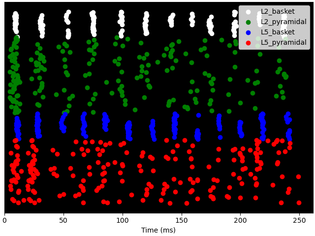
Take a look at how different cell types respond to the exogenous drive. Note the periodic firing pattern of all cell types. While the basket cells fire relatively synchronously, the pyramidal cell populations display a more varied pattern, in which only a fraction of cells reach firing threshold.

net.cell_response.plot_spikes_raster()

Out:

<Figure size 640x480 with 1 Axes>

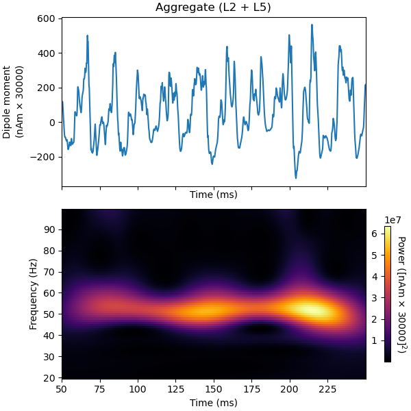
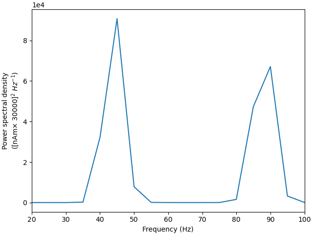
To confirm that the periodicity observed in the firing patterns correspond to a population oscillation in the gamma-range, we can plot the time-frequency representation together with the signal. Note that the network requires some time to reach steady state. Hence, we omit the first 50 ms in our analysis.

tmin = 50
trial_idx = 0  # pick first trial

# plot dipole time course and time-frequency representation in same figure
import numpy as np
import matplotlib.pyplot as plt

fig, axes = plt.subplots(2, 1, sharex=True, figsize=(6, 6),
                         constrained_layout=True)

dpls[trial_idx].plot(tmin=tmin, ax=axes[0], show=False)

# Create an fixed-step tiling of frequencies from 20 to 100 Hz in steps of 1 Hz
freqs = np.arange(20., 100., 1.)
dpls[trial_idx].plot_tfr_morlet(freqs, n_cycles=7, tmin=tmin, ax=axes[1])

Out:

<Figure size 600x600 with 3 Axes>

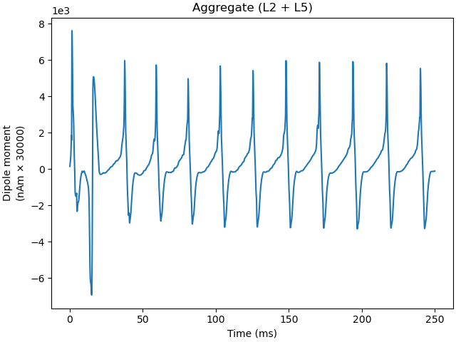
As a final exercise, let us try to re-run the simulation with a tonic bias applied to the L5 Pyramidal cells. Notice that the oscillation waveform is more regular, with less noise due to the fact that the tonic depolarization dominates over the influence of the Poisson drive. By default, a tonic bias is applied to the entire duration of the simulation.

net.add_tonic_bias(cell_type='L5_pyramidal', amplitude=6.)
dpls = simulate_dipole(net, n_trials=1)

dpls[trial_idx].plot()

Out:

joblib will run over 1 jobs
Building the NEURON model
[Done]
running trial 1 on 1 cores
Simulation time: 0.03 ms...
Simulation time: 10.0 ms...
Simulation time: 20.0 ms...
Simulation time: 30.0 ms...
Simulation time: 40.0 ms...
Simulation time: 50.0 ms...
Simulation time: 60.0 ms...
Simulation time: 70.0 ms...
Simulation time: 80.0 ms...
Simulation time: 90.0 ms...
Simulation time: 100.0 ms...
Simulation time: 110.0 ms...
Simulation time: 120.0 ms...
Simulation time: 130.0 ms...
Simulation time: 140.0 ms...
Simulation time: 150.0 ms...
Simulation time: 160.0 ms...
Simulation time: 170.0 ms...
Simulation time: 180.0 ms...
Simulation time: 190.0 ms...
Simulation time: 200.0 ms...
Simulation time: 210.0 ms...
Simulation time: 220.0 ms...
Simulation time: 230.0 ms...
Simulation time: 240.0 ms...

<Figure size 640x480 with 1 Axes>

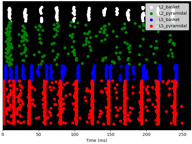
Notice that the Layer 5 pyramidal neurons now fire nearly synchronously, leading to a synchronous activation of the inhibitory basket neurons, resulting in a low-latency IPSP back onto the pyramidal cells. The duration of the IPSP is ~20 ms, after which the combined effect of the tonic bias and Poisson drive is to bring the pyramidal cells back to firing threshold, creating a ~50 Hz PING rhythm. This type of synchronous rhythm is sometimes referred to as “strong” PING.

net.cell_response.plot_spikes_raster()

Out:

<Figure size 640x480 with 1 Axes>

Although the simulated dipole signal demonstrates clear periodicity, its frequency is lower compared with the “weak” PING simulation above.

from hnn_core.viz import plot_psd
plot_psd(dpls[trial_idx], fmin=20., fmax=100., tmin=tmin)

Out:

<Figure size 640x480 with 1 Axes>

References

1(1,2)

Lee, S. & Jones, S. R. Distinguishing mechanisms of gamma frequency oscillations in human current source signals using a computational model of a laminar neocortical network. Frontiers in human neuroscience (2013)

2

https://jonescompneurolab.github.io/hnn-tutorials/gamma/gamma