01. Simulate dipole for evoked inputs

This example demonstrates how to simulate a dipole for evoked-like waveforms using HNN-core.

# Authors: Mainak Jas <mainak.jas@telecom-paristech.fr>
#          Sam Neymotin <samnemo@gmail.com>
#          Blake Caldwell <blake_caldwell@brown.edu>
#          Christopher Bailey <cjb@cfin.au.dk>

# sphinx_gallery_thumbnail_number = 2

import os.path as op
import tempfile

Let us import hnn_core

import hnn_core
from hnn_core import simulate_dipole, read_params, Network, read_spikes
from hnn_core.viz import plot_dipole

hnn_core_root = op.dirname(hnn_core.__file__)

Then we read the parameters file

params_fname = op.join(hnn_core_root, 'param', 'default.json')
params = read_params(params_fname)
print(params)

Out:

{
    "L2Basket_Gauss_A_weight": 0.0,
    "L2Basket_Gauss_mu": 2000.0,
    "L2Basket_Gauss_sigma": 3.6,
    "L2Basket_Pois_A_weight_ampa": 0.0,
    "L2Basket_Pois_A_weight_nmda": 0.0,
    "L2Basket_Pois_lamtha": 0.0,
    "L2Pyr_Gauss_A_weight": 0.0,
    "L2Pyr_Gauss_mu": 2000.0,
    "L2Pyr_Gauss_sigma": 3.6,
    "L2Pyr_Pois_A_weight_ampa": 0.0,
    "L2Pyr_Pois_A_weight_nmda": 0.0,
    "L2Pyr_Pois_lamtha": 0.0,
    "L2Pyr_ampa_e": 0.0,
    "L2Pyr_ampa_tau1": 0.5,
    "L2Pyr_ampa_tau2": 5.0,
    "L2Pyr_apical1_L": 306.0,
    "L2Pyr_apical1_diam": 4.08,
    "L2Pyr_apicaloblique_L": 340.0,
    "L2Pyr_apicaloblique_diam": 3.91,
    "L2Pyr_apicaltrunk_L": 59.5,
    "L2Pyr_apicaltrunk_diam": 4.25,
    "L2Pyr_apicaltuft_L": 238.0,
    "L2Pyr_apicaltuft_diam": 3.4,
    "L2Pyr_basal1_L": 85.0,
    "L2Pyr_basal1_diam": 4.25,
    "L2Pyr_basal2_L": 255.0,
    "L2Pyr_basal2_diam": 2.72,
    "L2Pyr_basal3_L": 255.0,
    "L2Pyr_basal3_diam": 2.72,
    "L2Pyr_dend_Ra": 200.0,
    "L2Pyr_dend_cm": 0.6195,
    "L2Pyr_dend_el_hh2": -65.0,
    "L2Pyr_dend_gbar_km": 250.0,
    "L2Pyr_dend_gkbar_hh2": 0.01,
    "L2Pyr_dend_gl_hh2": 4.26e-05,
    "L2Pyr_dend_gnabar_hh2": 0.15,
    "L2Pyr_gabaa_e": -80.0,
    "L2Pyr_gabaa_tau1": 0.5,
    "L2Pyr_gabaa_tau2": 5.0,
    "L2Pyr_gabab_e": -80.0,
    "L2Pyr_gabab_tau1": 1.0,
    "L2Pyr_gabab_tau2": 20.0,
    "L2Pyr_nmda_e": 0.0,
    "L2Pyr_nmda_tau1": 1.0,
    "L2Pyr_nmda_tau2": 20.0,
    "L2Pyr_soma_L": 22.1,
    "L2Pyr_soma_Ra": 200.0,
    "L2Pyr_soma_cm": 0.6195,
    "L2Pyr_soma_diam": 23.4,
    "L2Pyr_soma_el_hh2": -65.0,
    "L2Pyr_soma_gbar_km": 250.0,
    "L2Pyr_soma_gkbar_hh2": 0.01,
    "L2Pyr_soma_gl_hh2": 4.26e-05,
    "L2Pyr_soma_gnabar_hh2": 0.18,
    "L5Basket_Gauss_A_weight": 0.0,
    "L5Basket_Gauss_mu": 2000.0,
    "L5Basket_Gauss_sigma": 2.0,
    "L5Basket_Pois_A_weight_ampa": 0.0,
    "L5Basket_Pois_A_weight_nmda": 0.0,
    "L5Basket_Pois_lamtha": 0.0,
    "L5Pyr_Gauss_A_weight": 0.0,
    "L5Pyr_Gauss_mu": 2000.0,
    "L5Pyr_Gauss_sigma": 4.8,
    "L5Pyr_Pois_A_weight_ampa": 0.0,
    "L5Pyr_Pois_A_weight_nmda": 0.0,
    "L5Pyr_Pois_lamtha": 0.0,
    "L5Pyr_ampa_e": 0.0,
    "L5Pyr_ampa_tau1": 0.5,
    "L5Pyr_ampa_tau2": 5.0,
    "L5Pyr_apical1_L": 680.0,
    "L5Pyr_apical1_diam": 7.48,
    "L5Pyr_apical2_L": 680.0,
    "L5Pyr_apical2_diam": 4.93,
    "L5Pyr_apicaloblique_L": 255.0,
    "L5Pyr_apicaloblique_diam": 5.1,
    "L5Pyr_apicaltrunk_L": 102.0,
    "L5Pyr_apicaltrunk_diam": 10.2,
    "L5Pyr_apicaltuft_L": 425.0,
    "L5Pyr_apicaltuft_diam": 3.4,
    "L5Pyr_basal1_L": 85.0,
    "L5Pyr_basal1_diam": 6.8,
    "L5Pyr_basal2_L": 255.0,
    "L5Pyr_basal2_diam": 8.5,
    "L5Pyr_basal3_L": 255.0,
    "L5Pyr_basal3_diam": 8.5,
    "L5Pyr_dend_Ra": 200.0,
    "L5Pyr_dend_cm": 0.85,
    "L5Pyr_dend_el_hh2": -71.0,
    "L5Pyr_dend_gbar_ar": 1e-06,
    "L5Pyr_dend_gbar_ca": 60.0,
    "L5Pyr_dend_gbar_cat": 0.0002,
    "L5Pyr_dend_gbar_kca": 0.0002,
    "L5Pyr_dend_gbar_km": 200.0,
    "L5Pyr_dend_gkbar_hh2": 0.01,
    "L5Pyr_dend_gl_hh2": 4.26e-05,
    "L5Pyr_dend_gnabar_hh2": 0.14,
    "L5Pyr_dend_taur_cad": 20.0,
    "L5Pyr_gabaa_e": -80.0,
    "L5Pyr_gabaa_tau1": 0.5,
    "L5Pyr_gabaa_tau2": 5.0,
    "L5Pyr_gabab_e": -80.0,
    "L5Pyr_gabab_tau1": 1.0,
    "L5Pyr_gabab_tau2": 20.0,
    "L5Pyr_nmda_e": 0.0,
    "L5Pyr_nmda_tau1": 1.0,
    "L5Pyr_nmda_tau2": 20.0,
    "L5Pyr_soma_L": 39.0,
    "L5Pyr_soma_Ra": 200.0,
    "L5Pyr_soma_cm": 0.85,
    "L5Pyr_soma_diam": 28.9,
    "L5Pyr_soma_el_hh2": -65.0,
    "L5Pyr_soma_gbar_ar": 1e-06,
    "L5Pyr_soma_gbar_ca": 60.0,
    "L5Pyr_soma_gbar_cat": 0.0002,
    "L5Pyr_soma_gbar_kca": 0.0002,
    "L5Pyr_soma_gbar_km": 200.0,
    "L5Pyr_soma_gkbar_hh2": 0.01,
    "L5Pyr_soma_gl_hh2": 4.26e-05,
    "L5Pyr_soma_gnabar_hh2": 0.16,
    "L5Pyr_soma_taur_cad": 20.0,
    "N_pyr_x": 10,
    "N_pyr_y": 10,
    "N_trials": 1,
    "T_pois": -1,
    "celsius": 37.0,
    "dipole_scalefctr": 3000,
    "dipole_smooth_win": 30,
    "distribution_dist": "normal",
    "distribution_prox": "normal",
    "dt": 0.025,
    "dt_evprox0_evdist": -1,
    "dt_evprox0_evprox1": -1,
    "events_per_cycle_dist": 2,
    "events_per_cycle_prox": 2,
    "f_input_dist": 10.0,
    "f_input_prox": 10.0,
    "f_max_spec": 100,
    "f_stdev_dist": 20.0,
    "f_stdev_prox": 20.0,
    "gbar_L2Basket_L2Basket": 0.02,
    "gbar_L2Basket_L2Pyr_gabaa": 0.05,
    "gbar_L2Basket_L2Pyr_gabab": 0.05,
    "gbar_L2Basket_L5Pyr": 0.001,
    "gbar_L2Pyr_L2Basket": 0.0005,
    "gbar_L2Pyr_L2Pyr_ampa": 0.0005,
    "gbar_L2Pyr_L2Pyr_nmda": 0.0005,
    "gbar_L2Pyr_L5Basket": 0.00025,
    "gbar_L2Pyr_L5Pyr": 0.00025,
    "gbar_L5Basket_L5Basket": 0.02,
    "gbar_L5Basket_L5Pyr_gabaa": 0.025,
    "gbar_L5Basket_L5Pyr_gabab": 0.025,
    "gbar_L5Pyr_L5Basket": 0.0005,
    "gbar_L5Pyr_L5Pyr_ampa": 0.0005,
    "gbar_L5Pyr_L5Pyr_nmda": 0.0005,
    "gbar_evdist_1_L2Basket_ampa": 0.006562,
    "gbar_evdist_1_L2Basket_nmda": 0.019482,
    "gbar_evdist_1_L2Pyr_ampa": 7e-06,
    "gbar_evdist_1_L2Pyr_nmda": 0.004317,
    "gbar_evdist_1_L5Pyr_ampa": 0.1423,
    "gbar_evdist_1_L5Pyr_nmda": 0.080074,
    "gbar_evprox_1_L2Basket_ampa": 0.08831,
    "gbar_evprox_1_L2Basket_nmda": 0.0,
    "gbar_evprox_1_L2Pyr_ampa": 0.01525,
    "gbar_evprox_1_L2Pyr_nmda": 0.0,
    "gbar_evprox_1_L5Basket_ampa": 0.19934,
    "gbar_evprox_1_L5Basket_nmda": 0.0,
    "gbar_evprox_1_L5Pyr_ampa": 0.00865,
    "gbar_evprox_1_L5Pyr_nmda": 0.0,
    "gbar_evprox_2_L2Basket_ampa": 3e-06,
    "gbar_evprox_2_L2Basket_nmda": 0.0,
    "gbar_evprox_2_L2Pyr_ampa": 1.43884,
    "gbar_evprox_2_L2Pyr_nmda": 0.0,
    "gbar_evprox_2_L5Basket_ampa": 0.008958,
    "gbar_evprox_2_L5Basket_nmda": 0.0,
    "gbar_evprox_2_L5Pyr_ampa": 0.684013,
    "gbar_evprox_2_L5Pyr_nmda": 0.0,
    "inc_evinput": 0.0,
    "input_dist_A_delay_L2": 5.0,
    "input_dist_A_delay_L5": 5.0,
    "input_dist_A_weight_L2Basket_ampa": 0.0,
    "input_dist_A_weight_L2Basket_nmda": 0.0,
    "input_dist_A_weight_L2Pyr_ampa": 0.0,
    "input_dist_A_weight_L2Pyr_nmda": 0.0,
    "input_dist_A_weight_L5Pyr_ampa": 0.0,
    "input_dist_A_weight_L5Pyr_nmda": 0.0,
    "input_prox_A_delay_L2": 0.1,
    "input_prox_A_delay_L5": 1.0,
    "input_prox_A_weight_L2Basket_ampa": 0.0,
    "input_prox_A_weight_L2Basket_nmda": 0.0,
    "input_prox_A_weight_L2Pyr_ampa": 0.0,
    "input_prox_A_weight_L2Pyr_nmda": 0.0,
    "input_prox_A_weight_L5Basket_ampa": 0.0,
    "input_prox_A_weight_L5Basket_nmda": 0.0,
    "input_prox_A_weight_L5Pyr_ampa": 0.0,
    "input_prox_A_weight_L5Pyr_nmda": 0.0,
    "numspikes_evdist_1": 1,
    "numspikes_evprox_1": 1,
    "numspikes_evprox_2": 1,
    "prng_seedcore_evdist_1": 2,
    "prng_seedcore_evprox_1": 2,
    "prng_seedcore_evprox_2": 2,
    "prng_seedcore_extgauss": 2,
    "prng_seedcore_extpois": 2,
    "prng_seedcore_input_dist": 2,
    "prng_seedcore_input_prox": 2,
    "record_isoma": 0,
    "record_vsoma": 0,
    "repeats_dist": 10,
    "repeats_prox": 10,
    "save_dpl": 0,
    "save_figs": 0,
    "save_spec_data": 0,
    "sigma_t_evdist_1": 3.85,
    "sigma_t_evprox_1": 2.47,
    "sigma_t_evprox_2": 8.33,
    "sim_prefix": "default",
    "spec_cmap": "jet",
    "sync_evinput": false,
    "t0_input_dist": 1000,
    "t0_input_prox": 1000.0,
    "t0_input_stdev_dist": 0.0,
    "t0_input_stdev_prox": 0.0,
    "t0_pois": 0.0,
    "t_evdist_1": 63.53,
    "t_evprox_1": 26.61,
    "t_evprox_2": 137.12,
    "threshold": 0.0,
    "tstop": 170,
    "tstop_input_dist": 1001,
    "tstop_input_prox": 1001
}

This is a lot of parameters! We can also filter the parameters using unix-style wildcard characters. Most of the parameters relate to within-network connections and the cell geometry.

print(params['L2Pyr_soma*'])

Out:

{
    "L2Pyr_soma_L": 22.1,
    "L2Pyr_soma_Ra": 200.0,
    "L2Pyr_soma_cm": 0.6195,
    "L2Pyr_soma_diam": 23.4,
    "L2Pyr_soma_el_hh2": -65.0,
    "L2Pyr_soma_gbar_km": 250.0,
    "L2Pyr_soma_gkbar_hh2": 0.01,
    "L2Pyr_soma_gl_hh2": 4.26e-05,
    "L2Pyr_soma_gnabar_hh2": 0.18
}

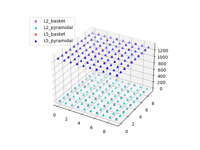
Let us first create our network from the params file and visualize the cells inside it.

net = Network(params)
net.plot_cells()

Out:

<Figure size 640x480 with 1 Axes>

The network of cells is now defined, to which we add external drives as required. Weights are prescribed separately for AMPA and NMDA receptors (receptors that are not used can be omitted or set to zero). The possible drive types include the following (click on the links for documentation):

• hnn_core.Network.add_evoked_drive()

• hnn_core.Network.add_poisson_drive()

• hnn_core.Network.add_bursty_drive()

First, we add a distal evoked drive

weights_ampa_d1 = {'L2_basket': 0.006562, 'L2_pyramidal': .000007,
                   'L5_pyramidal': 0.142300}
weights_nmda_d1 = {'L2_basket': 0.019482, 'L2_pyramidal': 0.004317,
                   'L5_pyramidal': 0.080074}
synaptic_delays_d1 = {'L2_basket': 0.1, 'L2_pyramidal': 0.1,
                      'L5_pyramidal': 0.1}
net.add_evoked_drive(
    'evdist1', mu=63.53, sigma=3.85, numspikes=1, weights_ampa=weights_ampa_d1,
    weights_nmda=weights_nmda_d1, location='distal',
    synaptic_delays=synaptic_delays_d1, seedcore=4)

Then, we add two proximal drives

weights_ampa_p1 = {'L2_basket': 0.08831, 'L2_pyramidal': 0.01525,
                   'L5_basket': 0.19934, 'L5_pyramidal': 0.00865}
synaptic_delays_prox = {'L2_basket': 0.1, 'L2_pyramidal': 0.1,
                        'L5_basket': 1., 'L5_pyramidal': 1.}
# all NMDA weights are zero; pass None explicitly
net.add_evoked_drive(
    'evprox1', mu=26.61, sigma=2.47, numspikes=1, weights_ampa=weights_ampa_p1,
    weights_nmda=None, location='proximal',
    synaptic_delays=synaptic_delays_prox, seedcore=4)

# Second proximal evoked drive. NB: only AMPA weights differ from first
weights_ampa_p2 = {'L2_basket': 0.000003, 'L2_pyramidal': 1.438840,
                   'L5_basket': 0.008958, 'L5_pyramidal': 0.684013}
# all NMDA weights are zero; omit weights_nmda (defaults to None)
net.add_evoked_drive(
    'evprox2', mu=137.12, sigma=8.33, numspikes=1,
    weights_ampa=weights_ampa_p2, location='proximal',
    synaptic_delays=synaptic_delays_prox, seedcore=4)

Now let’s simulate the dipole, running 2 trials with the Joblib backend. To run them in parallel we could set n_jobs to equal the number of trials. The Joblib backend allows running the simulations in parallel across trials.

from hnn_core import JoblibBackend

with JoblibBackend(n_jobs=1):
    dpls = simulate_dipole(net, n_trials=2, postproc=True)

Out:

joblib will run over 1 jobs
Loading custom mechanism files from /home/circleci/miniconda/envs/testenv/lib/python3.6/site-packages/hnn_core-0.1-py3.6.egg/hnn_core/mod/x86_64/.libs/libnrnmech.so
Building the NEURON model
[Done]
running trial 1 on 1 cores
Simulation time: 0.03 ms...
Simulation time: 10.0 ms...
Simulation time: 20.0 ms...
Simulation time: 30.0 ms...
Simulation time: 40.0 ms...
Simulation time: 50.0 ms...
Simulation time: 60.0 ms...
Simulation time: 70.0 ms...
Simulation time: 80.0 ms...
Simulation time: 90.0 ms...
Simulation time: 100.0 ms...
Simulation time: 110.0 ms...
Simulation time: 120.0 ms...
Simulation time: 130.0 ms...
Simulation time: 140.0 ms...
Simulation time: 150.0 ms...
Simulation time: 160.0 ms...
Building the NEURON model
[Done]
running trial 2 on 1 cores
Simulation time: 0.03 ms...
Simulation time: 10.0 ms...
Simulation time: 20.0 ms...
Simulation time: 30.0 ms...
Simulation time: 40.0 ms...
Simulation time: 50.0 ms...
Simulation time: 60.0 ms...
Simulation time: 70.0 ms...
Simulation time: 80.0 ms...
Simulation time: 90.0 ms...
Simulation time: 100.0 ms...
Simulation time: 110.0 ms...
Simulation time: 120.0 ms...
Simulation time: 130.0 ms...
Simulation time: 140.0 ms...
Simulation time: 150.0 ms...
Simulation time: 160.0 ms...

and then plot the amplitudes of the simulated aggregate dipole moments over time

import matplotlib.pyplot as plt
fig, axes = plt.subplots(2, 1, sharex=True, figsize=(6, 6),
                         constrained_layout=True)
plot_dipole(dpls, ax=axes[0], layer='agg', show=False)
net.cell_response.plot_spikes_hist(ax=axes[1],
                                   spike_types=['evprox', 'evdist'])

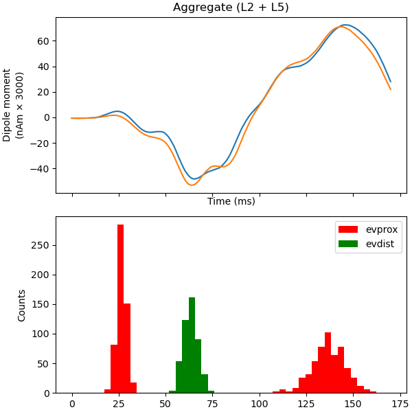
Out:

<Figure size 600x600 with 2 Axes>

Now, let us try to make the exogenous driving inputs to the cells synchronous and see what happens. This is achieved by setting the parameter sync_within_trial to True. Using the copy-method, we can create a clone of the network defined above, and then modify the drive dynamics for each drive. Making a copy removes any existing outputs from the network such as spiking information and voltages at the soma.

net_sync = net.copy()
net_sync.external_drives['evdist1']['dynamics']['sync_within_trial'] = True
net_sync.external_drives['evprox1']['dynamics']['sync_within_trial'] = True
net_sync.external_drives['evprox2']['dynamics']['sync_within_trial'] = True

You may interrogate current values defining the spike event time dynamics by

print(net_sync.external_drives['evdist1']['dynamics'])

Out:

{'mu': 63.53, 'sigma': 3.85, 'numspikes': 1, 'sync_within_trial': True}

Finally, let’s simulate this network.

dpls_sync = simulate_dipole(net_sync, n_trials=1)

trial_idx = 0
dpls_sync[trial_idx].plot()
net_sync.cell_response.plot_spikes_hist()

• 
• 

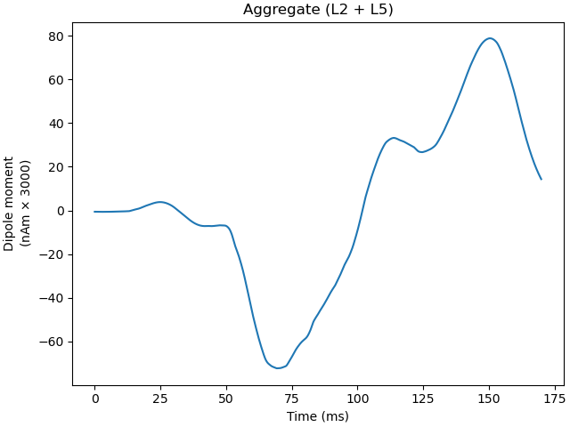
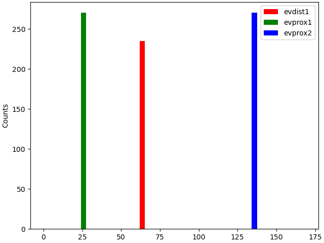
Out:

joblib will run over 1 jobs
Building the NEURON model
[Done]
running trial 1 on 1 cores
Simulation time: 0.03 ms...
Simulation time: 10.0 ms...
Simulation time: 20.0 ms...
Simulation time: 30.0 ms...
Simulation time: 40.0 ms...
Simulation time: 50.0 ms...
Simulation time: 60.0 ms...
Simulation time: 70.0 ms...
Simulation time: 80.0 ms...
Simulation time: 90.0 ms...
Simulation time: 100.0 ms...
Simulation time: 110.0 ms...
Simulation time: 120.0 ms...
Simulation time: 130.0 ms...
Simulation time: 140.0 ms...
Simulation time: 150.0 ms...
Simulation time: 160.0 ms...

<Figure size 640x480 with 1 Axes>