01. Simulate Event Related Potentials (ERPs)

This example demonstrates how to simulate a threshold level tactile evoked response, as detailed in the HNN GUI ERP tutorial, using HNN-core. We recommend you first review the GUI tutorial.

The workflow below recreates an example of the threshold level tactile evoked response, as observed in Jones et al. J. Neuroscience 2007 [1] (e.g. Figure 7 in the GUI tutorial), albeit without a direct comparison to the recorded data.

# Authors: Mainak Jas <mmjas@mgh.harvard.edu>
#          Sam Neymotin <samnemo@gmail.com>
#          Blake Caldwell <blake_caldwell@brown.edu>
#          Christopher Bailey <cjb@cfin.au.dk>

# sphinx_gallery_thumbnail_number = 3

import os.path as op
import tempfile

import matplotlib.pyplot as plt

Let us import hnn_core

import hnn_core
from hnn_core import simulate_dipole, jones_2009_model
from hnn_core.viz import plot_dipole

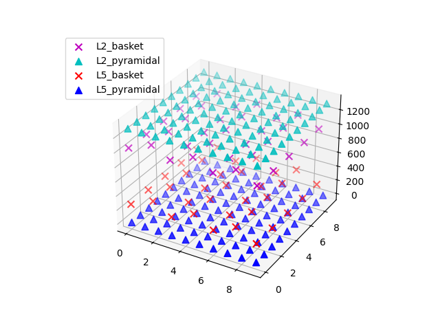
Let us first create our default network and visualize the cells inside it.

net = jones_2009_model()
net.plot_cells()
net.cell_types['L5_pyramidal'].plot_morphology()

• 
• 

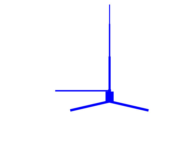
<Axes3D: >

The network of cells is now defined, to which we add external drives as required. Weights are prescribed separately for AMPA and NMDA receptors (receptors that are not used can be omitted or set to zero). The possible drive types include the following (click on the links for documentation):

• hnn_core.Network.add_evoked_drive()

• hnn_core.Network.add_poisson_drive()

• hnn_core.Network.add_bursty_drive()

First, we add a distal evoked drive

weights_ampa_d1 = {'L2_basket': 0.006562, 'L2_pyramidal': .000007,
                   'L5_pyramidal': 0.142300}
weights_nmda_d1 = {'L2_basket': 0.019482, 'L2_pyramidal': 0.004317,
                   'L5_pyramidal': 0.080074}
synaptic_delays_d1 = {'L2_basket': 0.1, 'L2_pyramidal': 0.1,
                      'L5_pyramidal': 0.1}
net.add_evoked_drive(
    'evdist1', mu=63.53, sigma=3.85, numspikes=1, weights_ampa=weights_ampa_d1,
    weights_nmda=weights_nmda_d1, location='distal',
    synaptic_delays=synaptic_delays_d1, event_seed=274)

Then, we add two proximal drives

weights_ampa_p1 = {'L2_basket': 0.08831, 'L2_pyramidal': 0.01525,
                   'L5_basket': 0.19934, 'L5_pyramidal': 0.00865}
synaptic_delays_prox = {'L2_basket': 0.1, 'L2_pyramidal': 0.1,
                        'L5_basket': 1., 'L5_pyramidal': 1.}
# all NMDA weights are zero; pass None explicitly
net.add_evoked_drive(
    'evprox1', mu=26.61, sigma=2.47, numspikes=1, weights_ampa=weights_ampa_p1,
    weights_nmda=None, location='proximal',
    synaptic_delays=synaptic_delays_prox, event_seed=544)

# Second proximal evoked drive. NB: only AMPA weights differ from first
weights_ampa_p2 = {'L2_basket': 0.000003, 'L2_pyramidal': 1.438840,
                   'L5_basket': 0.008958, 'L5_pyramidal': 0.684013}
# all NMDA weights are zero; omit weights_nmda (defaults to None)
net.add_evoked_drive(
    'evprox2', mu=137.12, sigma=8.33, numspikes=1,
    weights_ampa=weights_ampa_p2, location='proximal',
    synaptic_delays=synaptic_delays_prox, event_seed=814)

Now let’s simulate the dipole, running 2 trials with the Joblib backend. To run them in parallel we could set n_jobs to equal the number of trials. The Joblib backend allows running the simulations in parallel across trials.

from hnn_core import JoblibBackend

with JoblibBackend(n_jobs=2):
    dpls = simulate_dipole(net, tstop=170., n_trials=2)

Joblib will run 2 trial(s) in parallel by distributing trials over 2 jobs.

Rather than reading smoothing and scaling parameters from file, we recommend explicit use of the smooth() and scale() methods instead. Note that both methods operate in-place, i.e., the objects are modified.

window_len, scaling_factor = 30, 3000
for dpl in dpls:
    dpl.smooth(window_len).scale(scaling_factor)

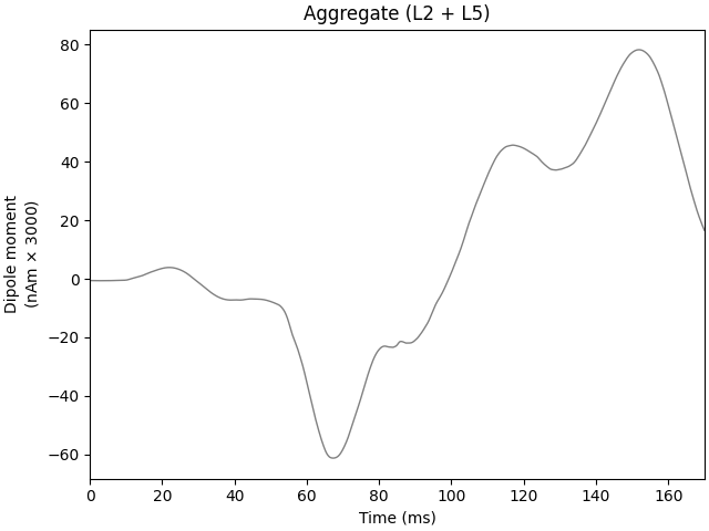
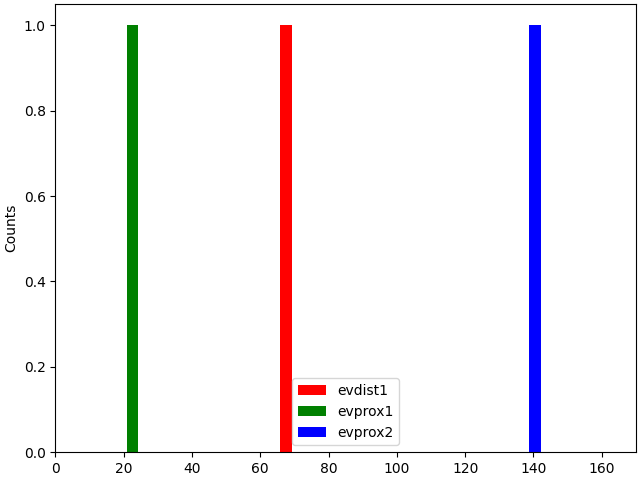
Plot the amplitudes of the simulated aggregate dipole moments over time

import matplotlib.pyplot as plt
fig, axes = plt.subplots(2, 1, sharex=True, figsize=(6, 6),
                         constrained_layout=True)
plot_dipole(dpls, ax=axes[0], layer='agg', show=False)
net.cell_response.plot_spikes_hist(ax=axes[1],
                                   spike_types=['evprox', 'evdist'])

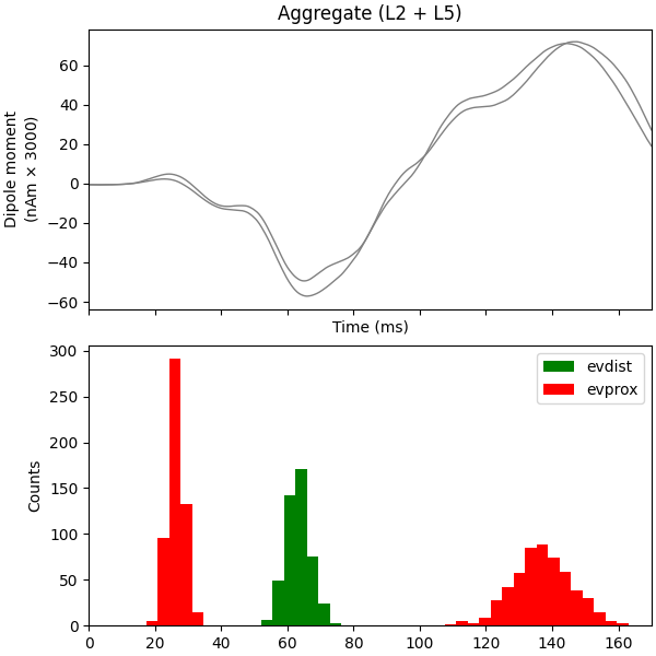
<Figure size 600x600 with 2 Axes>

If you want to analyze how the different cortical layers contribute to different net waveform features, then instead of passing 'agg' to layer, you can provide a list of layers to be visualized and optionally a list of axes to ax to visualize the dipole moments separately.

plot_dipole(dpls, average=False, layer=['L2', 'L5', 'agg'], show=False)

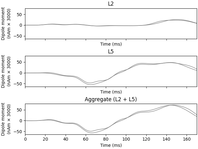
<Figure size 640x480 with 3 Axes>

Now, let us try to make the exogenous driving inputs to the cells synchronous and see what happens. This is achieved by setting n_drive_cells=1 and cell_specific=False when adding each drive.

net_sync = jones_2009_model()

n_drive_cells=1
cell_specific=False

net_sync.add_evoked_drive(
    'evdist1', mu=63.53, sigma=3.85, numspikes=1, weights_ampa=weights_ampa_d1,
    weights_nmda=weights_nmda_d1, location='distal', n_drive_cells=n_drive_cells,
    cell_specific=cell_specific, synaptic_delays=synaptic_delays_d1, event_seed=274)

net_sync.add_evoked_drive(
    'evprox1', mu=26.61, sigma=2.47, numspikes=1, weights_ampa=weights_ampa_p1,
    weights_nmda=None, location='proximal', n_drive_cells=n_drive_cells,
    cell_specific=cell_specific, synaptic_delays=synaptic_delays_prox, event_seed=544)

net_sync.add_evoked_drive(
    'evprox2', mu=137.12, sigma=8.33, numspikes=1,
    weights_ampa=weights_ampa_p2, location='proximal', n_drive_cells=n_drive_cells,
    cell_specific=cell_specific, synaptic_delays=synaptic_delays_prox, event_seed=814)

You may interrogate current values defining the spike event time dynamics by

print(net_sync.external_drives['evdist1']['dynamics'])

{'mu': 63.53, 'sigma': 3.85, 'numspikes': 1}

Finally, let’s simulate this network. Rather than modifying the dipole object, this time we make a copy of it before smoothing and scaling.

dpls_sync = simulate_dipole(net_sync, tstop=170., n_trials=1)

trial_idx = 0
dpls_sync[trial_idx].copy().smooth(window_len).scale(scaling_factor).plot()
net_sync.cell_response.plot_spikes_hist()

• 
• 

Joblib will run 1 trial(s) in parallel by distributing trials over 1 jobs.
Loading custom mechanism files from /Users/austinsoplata/rep/brn/hnn-core/hnn_core/mod/arm64/.libs/libnrnmech.so
Building the NEURON model
[Done]
Trial 1: 0.03 ms...
Trial 1: 10.0 ms...
Trial 1: 20.0 ms...
Trial 1: 30.0 ms...
Trial 1: 40.0 ms...
Trial 1: 50.0 ms...
Trial 1: 60.0 ms...
Trial 1: 70.0 ms...
Trial 1: 80.0 ms...
Trial 1: 90.0 ms...
Trial 1: 100.0 ms...
Trial 1: 110.0 ms...
Trial 1: 120.0 ms...
Trial 1: 130.0 ms...
Trial 1: 140.0 ms...
Trial 1: 150.0 ms...
Trial 1: 160.0 ms...

<Figure size 640x480 with 1 Axes>

Warning

• Always look at dipoles in conjunction with raster plots and spike histogram to avoid misinterpretation.

• Run multiple trials of your simulation to get an average of different drives seeds before drawing conclusions.

References

[1]

Jones, Stephanie R., et al. “Neural correlates of tactile detection: a combined magnetoencephalography and biophysically based computational modeling study.” Journal of Neuroscience 27.40 (2007): 10751-10764.