07. Batch Simulation

This example shows how to do batch simulations in HNN-core, allowing users to efficiently run multiple simulations with different parameters for comprehensive analysis.

# Authors: Abdul Samad Siddiqui <abdulsamadsid1@gmail.com>
#          Nick Tolley <nicholas_tolley@brown.edu>
#          Ryan Thorpe <ryan_thorpe@brown.edu>
#          Mainak Jas <mjas@mgh.harvard.edu>

Let us import hnn_core.

import matplotlib.pyplot as plt
import numpy as np
from hnn_core.batch_simulate import BatchSimulate
from hnn_core import jones_2009_model

# The number of cores may need modifying depending on your current machine.
n_jobs = 10

def set_params(param_values, net=None):
    """
    Set parameters in the network drives.

    Parameters
    ----------
    param_values : dict
        Dictionary of parameter values.
    net : instance of Network, optional
        If None, a new network is created using the specified model type.
    """
    weights_ampa = {'L2_basket': param_values['weight_basket'],
                    'L2_pyramidal': param_values['weight_pyr'],
                    'L5_basket': param_values['weight_basket'],
                    'L5_pyramidal': param_values['weight_pyr']}

    synaptic_delays = {'L2_basket': 0.1, 'L2_pyramidal': 0.1,
                       'L5_basket': 1., 'L5_pyramidal': 1.}

    # Add an evoked drive to the network.
    net.add_evoked_drive('evprox',
                         mu=40,
                         sigma=5,
                         numspikes=1,
                         location='proximal',
                         weights_ampa=weights_ampa,
                         synaptic_delays=synaptic_delays)

Define a parameter grid for the batch simulation.

param_grid = {
    'weight_basket': np.logspace(-4 - 1, 10),
    'weight_pyr': np.logspace(-4, -1, 10)
}

Define a function to calculate summary statistics

def summary_func(results):
    """
    Calculate the min and max dipole peak for each simulation result.

    Parameters
    ----------
    results : list
        List of dictionaries containing simulation results.

    Returns
    -------
    summary_stats : list
        Summary statistics for each simulation result.
    """
    summary_stats = []
    for result in results:
        dpl_smooth = result['dpl'][0].copy().smooth(window_len=30)
        dpl_data = dpl_smooth.data['agg']
        min_peak = np.min(dpl_data)
        max_peak = np.max(dpl_data)
        summary_stats.append({'min_peak': min_peak, 'max_peak': max_peak})
    return summary_stats

Run the batch simulation and collect the results.

# Comment off this code, if dask and distributed Python packages are installed
# from dask.distributed import Client
# client = Client(threads_per_worker=1, n_workers=5, processes=False)


# Run the batch simulation and collect the results.
net = jones_2009_model(mesh_shape=(3, 3))
batch_simulation = BatchSimulate(net=net,
                                 set_params=set_params,
                                 summary_func=summary_func)
simulation_results = batch_simulation.run(param_grid,
                                          n_jobs=n_jobs,
                                          combinations=False,
                                          backend='multiprocessing')
# backend='dask' if installed
print("Simulation results:", simulation_results)

[Parallel(n_jobs=10)]: Using backend MultiprocessingBackend with 10 concurrent workers.
[Parallel(n_jobs=10)]: Done   1 tasks      | elapsed:    2.4s
[Parallel(n_jobs=10)]: Using backend MultiprocessingBackend with 10 concurrent workers.
[Parallel(n_jobs=10)]: Done   1 tasks      | elapsed:    2.4s
[Parallel(n_jobs=10)]: Using backend MultiprocessingBackend with 10 concurrent workers.
[Parallel(n_jobs=10)]: Done   1 tasks      | elapsed:    2.4s
[Parallel(n_jobs=10)]: Using backend MultiprocessingBackend with 10 concurrent workers.
[Parallel(n_jobs=10)]: Done   1 tasks      | elapsed:    2.4s
[Parallel(n_jobs=10)]: Using backend MultiprocessingBackend with 10 concurrent workers.
[Parallel(n_jobs=10)]: Done   1 tasks      | elapsed:    2.4s
[Parallel(n_jobs=10)]: Using backend MultiprocessingBackend with 10 concurrent workers.
[Parallel(n_jobs=10)]: Done   1 tasks      | elapsed:    2.4s
[Parallel(n_jobs=10)]: Using backend MultiprocessingBackend with 10 concurrent workers.
[Parallel(n_jobs=10)]: Done   1 tasks      | elapsed:    2.4s
[Parallel(n_jobs=10)]: Using backend MultiprocessingBackend with 10 concurrent workers.
[Parallel(n_jobs=10)]: Done   1 tasks      | elapsed:    2.4s
[Parallel(n_jobs=10)]: Using backend MultiprocessingBackend with 10 concurrent workers.
[Parallel(n_jobs=10)]: Done   1 tasks      | elapsed:    2.4s
[Parallel(n_jobs=10)]: Using backend MultiprocessingBackend with 10 concurrent workers.
[Parallel(n_jobs=10)]: Done   1 tasks      | elapsed:    2.3s
Simulation results: {'summary_statistics': [[{'min_peak': -1.9487233699162363e-05, 'max_peak': 2.4382998111724826e-05}], [{'min_peak': -1.9487233699162363e-05, 'max_peak': 5.4069612580043786e-05}], [{'min_peak': -1.9487233699162363e-05, 'max_peak': 0.00011922352353898096}], [{'min_peak': -0.0006636604554164356, 'max_peak': 0.001140464508904066}], [{'min_peak': -1.9487233699162363e-05, 'max_peak': 0.0009097461915339884}], [{'min_peak': -1.9487233699162363e-05, 'max_peak': 0.001136209593608592}], [{'min_peak': -1.9487233699162363e-05, 'max_peak': 0.0011684582303501953}], [{'min_peak': -1.9487233699162363e-05, 'max_peak': 0.0012737618628301754}], [{'min_peak': -1.9487233699162363e-05, 'max_peak': 0.0014391544369764242}], [{'min_peak': -1.9487233699162363e-05, 'max_peak': 0.0016169395528490681}]], 'simulated_data': [[{'net': <Network | 3 x 3 Pyramidal cells (L2, L5)
3 L2 basket cells
3 L5 basket cells>, 'param_values': {'weight_basket': 1e-05, 'weight_pyr': 0.0001}, 'dpl': [<hnn_core.dipole.Dipole object at 0x7f44f912ca30>]}], [{'net': <Network | 3 x 3 Pyramidal cells (L2, L5)
3 L2 basket cells
3 L5 basket cells>, 'param_values': {'weight_basket': 2.0235896477251556e-05, 'weight_pyr': 0.00021544346900318845}, 'dpl': [<hnn_core.dipole.Dipole object at 0x7f44f912e0b0>]}], [{'net': <Network | 3 x 3 Pyramidal cells (L2, L5)
3 L2 basket cells
3 L5 basket cells>, 'param_values': {'weight_basket': 4.094915062380427e-05, 'weight_pyr': 0.00046415888336127773}, 'dpl': [<hnn_core.dipole.Dipole object at 0x7f44f912ee00>]}], [{'net': <Network | 3 x 3 Pyramidal cells (L2, L5)
3 L2 basket cells
3 L5 basket cells>, 'param_values': {'weight_basket': 8.286427728546843e-05, 'weight_pyr': 0.001}, 'dpl': [<hnn_core.dipole.Dipole object at 0x7f44f912fc40>]}], [{'net': <Network | 3 x 3 Pyramidal cells (L2, L5)
3 L2 basket cells
3 L5 basket cells>, 'param_values': {'weight_basket': 0.00016768329368110083, 'weight_pyr': 0.002154434690031882}, 'dpl': [<hnn_core.dipole.Dipole object at 0x7f44f912d210>]}], [{'net': <Network | 3 x 3 Pyramidal cells (L2, L5)
3 L2 basket cells
3 L5 basket cells>, 'param_values': {'weight_basket': 0.000339322177189533, 'weight_pyr': 0.004641588833612777}, 'dpl': [<hnn_core.dipole.Dipole object at 0x7f44f912d480>]}], [{'net': <Network | 3 x 3 Pyramidal cells (L2, L5)
3 L2 basket cells
3 L5 basket cells>, 'param_values': {'weight_basket': 0.0006866488450042998, 'weight_pyr': 0.01}, 'dpl': [<hnn_core.dipole.Dipole object at 0x7f44c0d437c0>]}], [{'net': <Network | 3 x 3 Pyramidal cells (L2, L5)
3 L2 basket cells
3 L5 basket cells>, 'param_values': {'weight_basket': 0.0013894954943731374, 'weight_pyr': 0.021544346900318822}, 'dpl': [<hnn_core.dipole.Dipole object at 0x7f44c0d40250>]}], [{'net': <Network | 3 x 3 Pyramidal cells (L2, L5)
3 L2 basket cells
3 L5 basket cells>, 'param_values': {'weight_basket': 0.002811768697974231, 'weight_pyr': 0.046415888336127774}, 'dpl': [<hnn_core.dipole.Dipole object at 0x7f44c0d435b0>]}], [{'net': <Network | 3 x 3 Pyramidal cells (L2, L5)
3 L2 basket cells
3 L5 basket cells>, 'param_values': {'weight_basket': 0.005689866029018299, 'weight_pyr': 0.1}, 'dpl': [<hnn_core.dipole.Dipole object at 0x7f44c0d41840>]}]]}

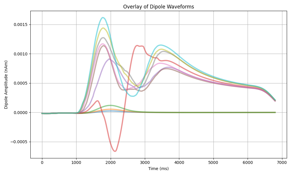
This plot shows an overlay of all smoothed dipole waveforms from the batch simulation. Each line represents a different set of parameters, allowing us to visualize the range of responses across the parameter space.

dpl_waveforms = []
for data_list in simulation_results['simulated_data']:
    for data in data_list:
        dpl_smooth = data['dpl'][0].copy().smooth(window_len=30)
        dpl_waveforms.append(dpl_smooth.data['agg'])

plt.figure(figsize=(10, 6))
for waveform in dpl_waveforms:
    plt.plot(waveform, alpha=0.5, linewidth=3)
plt.title('Overlay of Dipole Waveforms')
plt.xlabel('Time (ms)')
plt.ylabel('Dipole Amplitude (nAm)')
plt.grid(True)
plt.tight_layout()
plt.show()

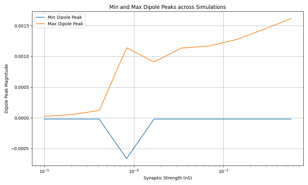
This plot displays the minimum and maximum dipole peaks across different synaptic strengths. This allows us to see how the range of dipole activity changes as we vary the synaptic strength parameter.

min_peaks, max_peaks, param_values = [], [], []
for summary_list, data_list in zip(simulation_results['summary_statistics'],
                                   simulation_results['simulated_data']):
    for summary, data in zip(summary_list, data_list):
        min_peaks.append(summary['min_peak'])
        max_peaks.append(summary['max_peak'])
        param_values.append(data['param_values']['weight_basket'])

# Plotting
plt.figure(figsize=(10, 6))
plt.plot(param_values, min_peaks, label='Min Dipole Peak')
plt.plot(param_values, max_peaks, label='Max Dipole Peak')
plt.xlabel('Synaptic Strength (nS)')
plt.ylabel('Dipole Peak Magnitude')
plt.title('Min and Max Dipole Peaks across Simulations')
plt.legend()
plt.grid(True)
plt.xscale('log')
plt.tight_layout()
plt.show()