06. Animating HNN simulations

This example demonstrates how to animate HNN simulations

# Author: Nick Tolley <nicholas_tolley@brown.edu>

First, we’ll import the necessary modules for instantiating a network and running a simulation that we would like to animate.

import os.path as op

import hnn_core
from hnn_core import jones_2009_model, simulate_dipole, read_params
from hnn_core.network_models import add_erp_drives_to_jones_model

We begin by instantiating the network. For this example, we will reduce the number of cells in the network to speed up the simulations.

net = jones_2009_model(mesh_shape=(3, 3))

# Note that we move the cells further apart to allow better visualization of
# the network (default inplane_distance=1.0 µm).
net.set_cell_positions(inplane_distance=300)

The hnn_core.viz.NetworkPlotter class can be used to visualize the 3D structure of the network.

from hnn_core.viz import NetworkPlotter

net_plot = NetworkPlotter(net)
net_plot.fig

/home/circleci/miniconda/envs/testenv/lib/python3.8/site-packages/hnn_core/viz.py:962: UserWarning: The figure layout has changed to tight
  plt.tight_layout()

<Figure size 640x480 with 2 Axes>

We can also visualize the network from another angle by adjusting the azimuth and elevation parameters.

net_plot.azim = 45
net_plot.elev = 40
net_plot.fig

<Figure size 640x480 with 2 Axes>

Next we add event related potential (ERP) producing drives to the network and run the simulation (see evoked example for more details). To visualize the membrane potential of cells in the network, we need use simulate_dipole(…, record_vsec=’all’) which turns on the recording of voltages in all sections of all cells in the network.

add_erp_drives_to_jones_model(net)
dpl = simulate_dipole(net, tstop=170, record_vsec='all')
net_plot = NetworkPlotter(net)  # Reinitialize plotter with simulated network

Joblib will run 1 trial(s) in parallel by distributing trials over 1 jobs.
Building the NEURON model
[Done]
Trial 1: 0.03 ms...
Trial 1: 10.0 ms...
Trial 1: 20.0 ms...
Trial 1: 30.0 ms...
Trial 1: 40.0 ms...
Trial 1: 50.0 ms...
Trial 1: 60.0 ms...
Trial 1: 70.0 ms...
Trial 1: 80.0 ms...
Trial 1: 90.0 ms...
Trial 1: 100.0 ms...
Trial 1: 110.0 ms...
Trial 1: 120.0 ms...
Trial 1: 130.0 ms...
Trial 1: 140.0 ms...
Trial 1: 150.0 ms...
Trial 1: 160.0 ms...

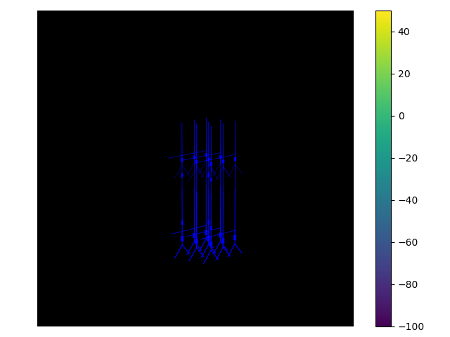
Finally, we can animate the simulation using the export_movie() method. We can adjust the xyz limits of the plot to better visualize the network.

net_plot.xlim = (400, 1600)
net_plot.ylim = (400, 1600)
net_plot.zlim = (-500, 1600)
net_plot.azim = 225
net_plot.export_movie('animation_demo.gif', dpi=100, fps=30, interval=100)

<matplotlib.animation.FuncAnimation object at 0x7f5da8b57eb0>