
Tutorials
HNN release 1.0 provides an automated model optimization tool that can be used to efficiently estimate parameter values that will minimize the error between model output and features of experimental ERP waveforms. The optimization tool is designed to efficiently arrive at parameter estimates without the need for supercomputing or high-performance resources. We leverage two insights to reduce the number of simulations needed for optimization. First, the key parameters of ERP generation are reslated to the “activation” of the network (i.e. exogenous/evoked inputs). So these are the only parameters estimated. Second, results from our sensitivity analyses have shown that the parameters of a particular input will have their most prominent effect on features of the dipole waveform that occur after the input’s onset, but the effect decays as later inputs begin impacting the dipole as well. We combine these insights in a stepwise optimization procedure that can be accessed through the HNN GUI. For more details on the tool and its stepwise input optimization process, please see [1].
The rest of this tutorial demonstrates how HNN’s optimization tool can be used to estimate parameters for ERP simulations, resulting in a better match to experimental data. Before starting an optimization, users must supply a baseline configuration that includes the number and type of hypothesized evoked inputs and the approximate timing of each input. Users may use one of the parameter files included with HNN as a baseline or use the GUI to interactively add and remove evoked inputs to arrive at a suitable starting point for optimization. A future feature planned for HNN will attempt to automate this task based on the number of maxima and minima in the waveform. For now, users should use the timing of these features in the waveform to estimate the type (proximal/distal) and timing of evoked inputs.
After completing the optimization of evoked inputs from a parameter file to match new experimental data, the tutorial will cover refining the original optimization and then using the optimized values to identify the key parameters responsible for the improved fit.
We start from the ERP example used in the previous Evoked potentials tutorial. The tutorial began with a parameter set from an experimental paradigm of an ERP source-localized to the somatosensory cortex, which was elicited from a perceptual threshold-level stimulation – 50% detected. The tutorial then introduced the suprathreshold case – 100% detected – which had a different early ERP waveform. Here, we will explore the differences between these two cases in more detail, starting with simulation parameters tuned for the 50% scenario and using the automated model optimization tool to arrive at parameters that fit the 100% detected suprathreshold data.
Figure 1 shows the dipole output of an HNN model with parameters from the perceptual threshold-level stimulation example. Only 3 trials are run in the examples part of this tutorial. To produce Figure 1 yourself, start by removing the default parameter file going to the Simulation drop-down menu and selecting “Clear simulation(s)”. The click “Set Parameters From File” button on the main menu and select the parameter file “ERPYes100Trials.param”. This file should be visible in the default directory, but you can find it under the “hnn_source_code” directory and then “param”. Now change some simulation parameters by clicking on “Set Parameters” and first changing the “Simulation Name” to “ERPYes3Trials”. Next click the “Run” button and change “Trials” to 3. Now load the data file “yes_trial_S1_ERP_all_avg.txt” by going back to the main window and from the “File” drop-down menu, select “Load data file”. The file can be found under the “MEG_detection_data” folder. Finally, click “Run Simulation” to initiate the 3 trial simulation.
The very low RMSE of 5.02 is because these parameters were tuned to match the “yes_trial_S1_ERP_all_avg” data. Having the parameters that result in a simulation matched to the experimental data allows users to develop their own hypotheses and make inferences on the dynamics responsible for producing the ERP waveform observed in the experiment.
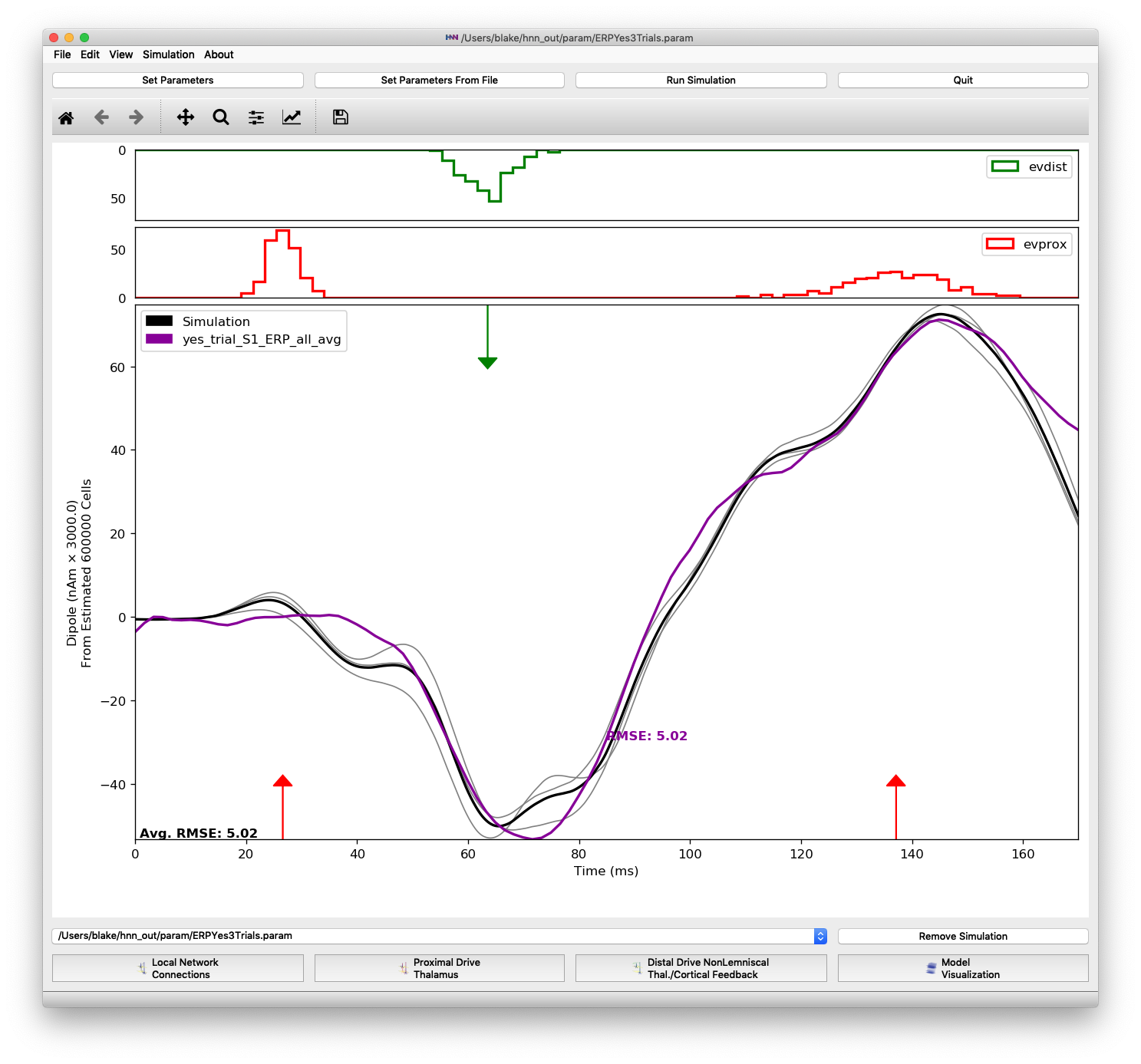
Simulation of perceptual threshold-level stimulation parameter set over 3 trials, matched to experimental data.
However, HNN users may be interested in making inferences on the dynamics underlying different experimental paradigms or even different cortical areas. We will now look at a suprathreshold stimulation scenario and using automated model optimization to match the simulation to new data. In later sections, we will explore what circuit-level parameters changes were significant in matching the new data.
Remove the “yes_trial_S1_ERP_all_avg” data plot from the main HNN window by clicking on the File drop-down menu and selecting “Clear data file(s)”. Then load the suprathreshold data “S1_SupraT.txt” from File->“Load data file”.
The plot below shows the differences between the threshold-level simulation and the suprathreshold data. The RMSE between the old simulation output and the suprathreshold data is much higher, now 30.53, indicating a poor fit between simulation parameters and the experimental data.

Simulation run with parameters for the perceptual threshold-level scenario plotted against the longer duration suprathreshold-level experimental data
Also, note that the “S1_SupraT” experimental data extends further in duration than the “yes_trial_S1_ERP_all_avg” data shown previously. We can simulate the full length of the suprathreshold data by changing the simulation duration. Click the “Set Parameters button”, then the “Run” button, and change the duration to 173.325 ms as shown in Figure 3.
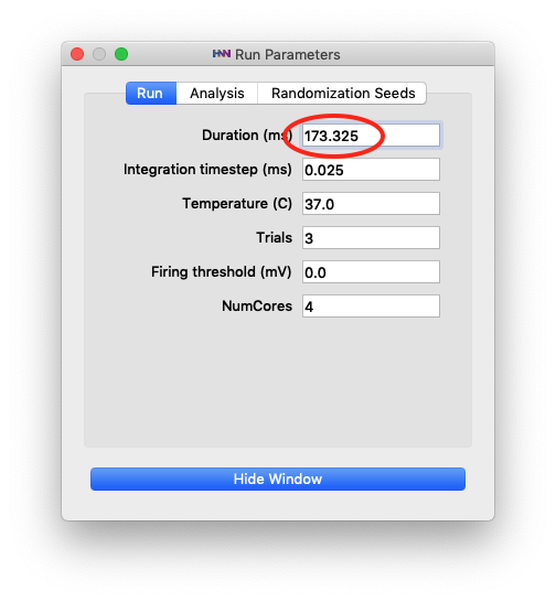
Run Parameters dialog box
Also, change the “Simulation Name” to “ERPYes3Trials_173ms_opt” so that the optimized parameters will be saved in their own file (when we run it later). Next click “Run Simulation” button to obtain an updated RMSE for 3 trials over the 173.325 ms simulation. We can see in the plots of main HNN window that the simulation runs for the full duration of the suprathreshold data that we are comparing to.
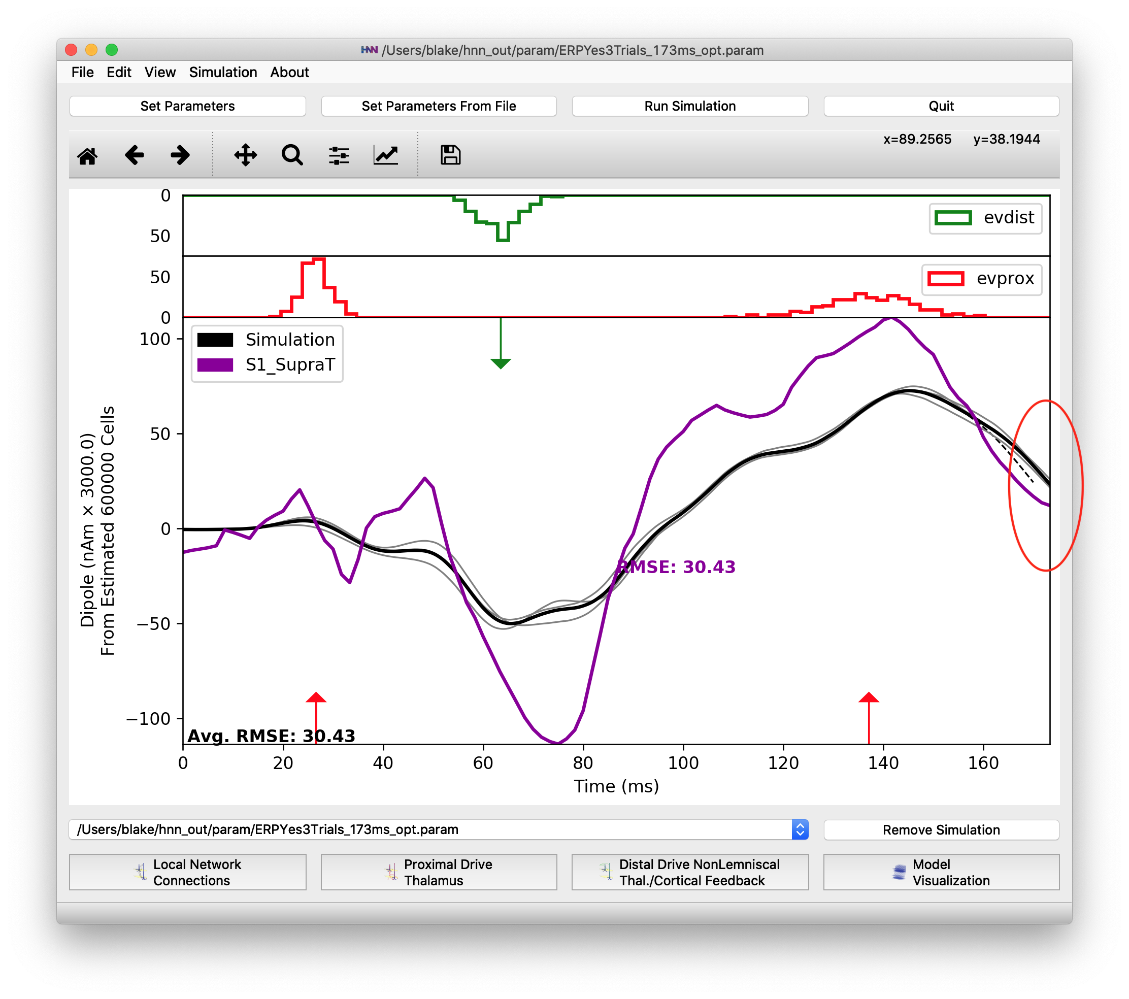
Full 173.325 ms simulation using the parameters for the 50% detection scenario.
Once both data and parameter files have been loaded, the “Configure Optimization” menu selection will become available under the “Simulation” drop-down menu. Click on this selection to open up the “Configure Optimization” dialog box shown in Figure 5.
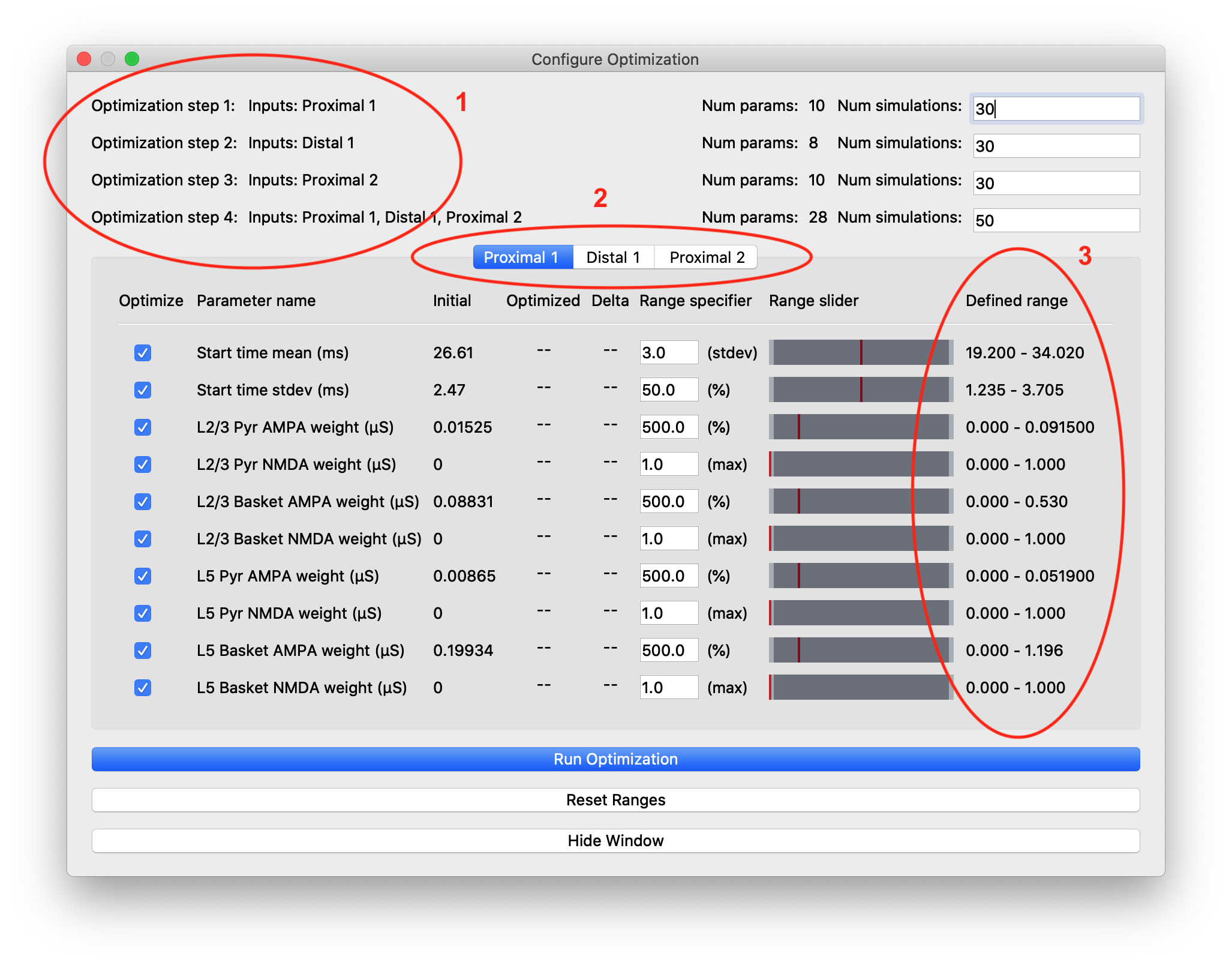
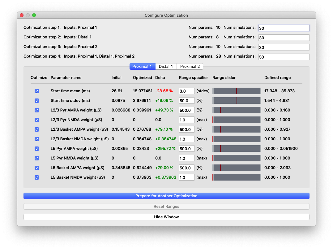
“Configure Optimization” dialog box with different areas highlighted: 1) Listing of the optimization steps for each evoked input. When inputs are combined in a single step, they are shown on a single line here. The user can configure the number of simulations for each step. 2) Tabs to navigate to the parameters and configurable optimization range for each evoked input. 3) The range over which the optimization algorithm will search for each parameter is calculated from user-specified multiplier and is displayed in the right-most column.
The upper portion of this dialog box contains configuration information for the stepwise optimization procedure and displays the inputs and parameters that will be optimized in each step. In the parameter file we are using for somatosensory ERPs, there are three evoked inputs defined, each of which is targeted in a step of the optimization procedure. During each step, the optimization will minimize a weighted RMSE measure that prioritizes the errors at time points that are most likely to be affected by input parameter changes. The last optimization step varies all parameters at once and is designed to minimize downstream effects that might arise from overfitting earlier features of the waveform at the expense of the fit later in the simulation. The default number of simulations for each step was chosen to provide a significantly improved fit, but keep the overall time required by the optimization within an hour, even on a laptop.
The tabs of the dialog box are organized by evoked input and show the input parameters in rows along with the range used by the optimization algorithm in searching for parameter estimates. We use the COBYLA algorithm [2] implemented in the nlopt Python package
The user-specified field “Range specifier” can be modified to widen or narrow the parameter search if additional insights into reasonable values are known ahead of time. The user can move the ends of the “Range slider” using the mouse to choose an asymmetric parameter range. The initial value is shown with a red line, allowing the user to easily define a range above or below the initial value, for example. Pressing the “Reset Ranges” button will reset the slider and display updated values in the “Defined range” column.
Leave all parameters enabled for optimization (checked) and press the “Run Optimization” button to begin the procedure. Depending on your system, it will take between up to 2 hours to finish. A MacBook Pro with an 8-core 2.3 Ghz processor takes about 35 minute to complete an optimization round.
You can monitor the progress in the “View Simulation Log” dialog box. The output will indicate what step and simulation is currently being run and the dipole plot in the main HNN window will be updated after each step has completed. Note that the first steps do not require a full simulation, because the weighted RMSE is insignificant at later points. In the dipole plots, HNN will only display normal (non-weighted RMSE).
While the optimization is in progress, you can make changes to parameter ranges or select/deselect parameters for inputs that will be optimized in a later step. Once the optimization of an input has begun, its parameters will be grayed out for the remainder of the optimization round.
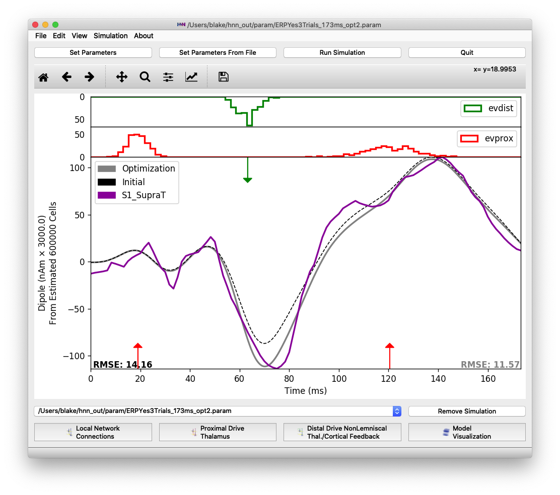
After all optimization steps complete, you will see a plot similar to Figure 6, where the optimized fit will be shown in gray with the initial fit (before optimization) marked by a dashed black line. We can see that the model optimization reduced overall RMSE from 30.43 to 14.16. The amplitudes of the trough at 70 ms and the peak at 135 ms were increased. However, we will seek to improve upon this fit in the sections below.
It is interesting to note that the optimization chose mean start time values for each input that were earlier to better match suprathreshold data. The weights of almost every synaptic connection also increased during optimization. These changes are consistent with a hypothesis that the circuit-level inputs from a suprathreshold stimulus come faster and stronger than a threshold-level stimulus detected 50% of the time.

The first round of automated parameter optimization reduces the RMSE from 30.43 to 14.16. RMSE is calculated as the difference between the average of 3 trials and suprathreshold experimental data.
|
|
|
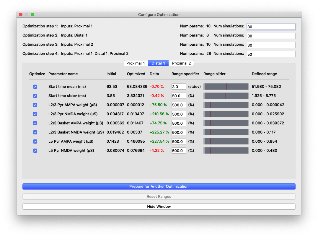
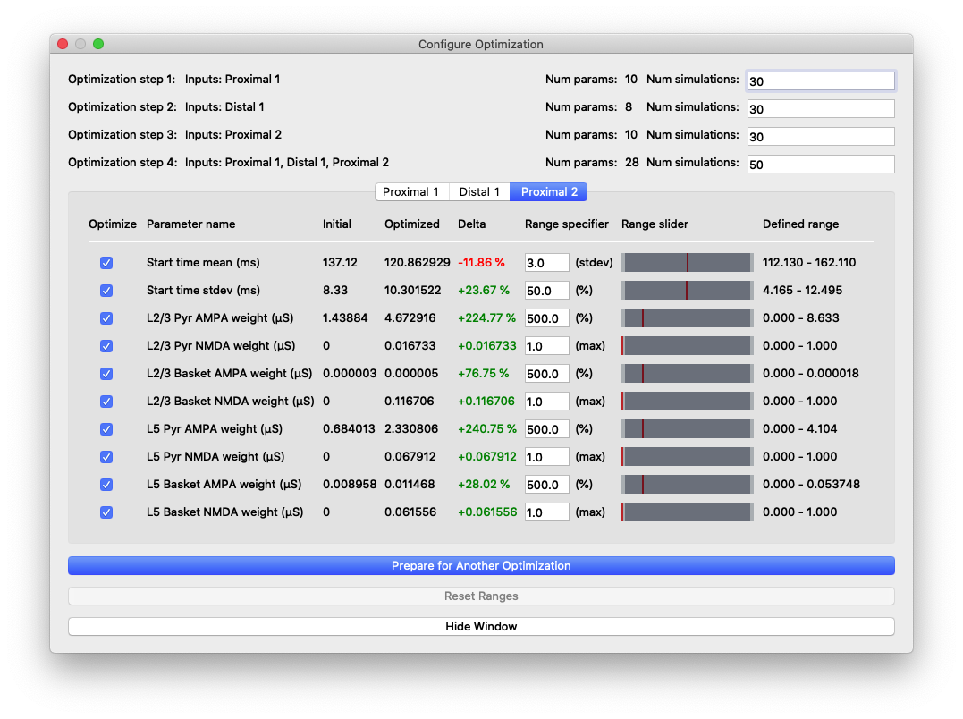
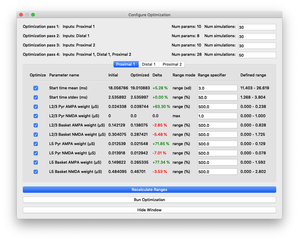
Parameter values and relative changes in the first optimization shown in Figure 6.
While the fit shown in Figure 6 is significantly improved over the baseline parameters, we haven’t yet achieved the same level of fit with the suprathreshold data that we had with the threshold-level data (RMSE 5.02). One explanation may be that the default ranges limited parameter exploration, missing the optimal values. Additionally, the number of simulations could have been insufficient to sample the high-dimensional parameter space.
The parameter changes shown in Figure 7 in green and red indicate that the parameter search may have been limiting. In fact, the COBYLA algorithm starts with parameter changes of 75% before conservatively increasing the range of the parameter search. So a change of 200% (Distal 1) may have been the largest change explored in our limited number of simulation. To see if these parameters were limited by the ranges, we perform more optimization rounds below. Note that you may want to skip performing these yourself, depending on your processor speed and number of cores. Without running an optimization round, you can proceed through this tutorial by just examining the resulting parameter values in the “Optimized” column of the “Configure Optimization” dialogs shown below.
Running a second optimization results a better fit in the region characterized by the large negative trough, and overall RMSE drops to 14.07. However, several parameters did not change as much as in the first optimization. One that continued to increase by over 200% was the layer 2/3 pyramidal NMDA weight for the distal 1 input.
A second optimization round reducing RMSE from 17.65 to 14.07
|
|

|
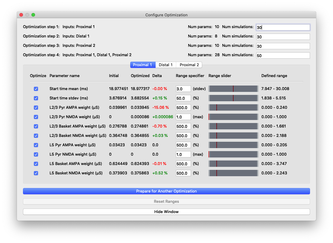
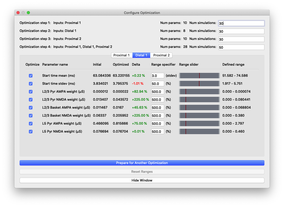
Parameter values and relative changes in the optimization shown in Figure 8.
We performed a third optimization round with the resultant fit shown in Figure 10. Finally, the simulation output matches the negative trough in the experimental data well and RMSE is reduced to 10.40. We can see that the layer 2/3 pyramidal NMDA weight for the distal 1 input increased again, by 174% this time. At this point, it has changed over 2500% from its baseline value. This large change requires the user to pause to examine whether the new value is physiologically plausible or rather if the model is being overfitted to data. The user must go back to the original hypothesis and assess whether the changes made by parameter optimization are consistent. If not, the observation that such large changes were necessary could hint towards a new hypothesis that would better explain experimental data.
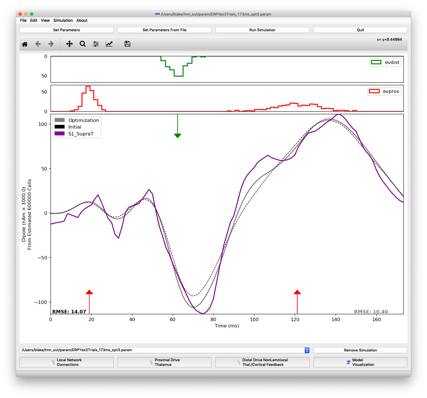
A third optimization round reducing RMSE from 14.07 to 10.40
|

|
|
Parameter values and relative changes in the optimization shown in Figure 10.
Even though our optimization has dropped the simulation’s RMSE compared to the suprathreshold data to 10.40, we are still using a large smoothing window (the default for perceptual-level threshold simulations) of 30 ms. The suprathreshold data has sharper features that we may want to optimize to, notably the second small peak between the first proximal and distal inputs. To explore what the simulation output looks like with a smaller smoothing window, click “Set Parameters” -> “Run”, select the “Analysis” tab and then enter 15 for “Dipole Smooth Window (ms)”. Change the simulation name to indicate that smoothing has changed (e.g. append “window_15ms”), and then click “Run Simulation” to see the output. As expected, RMSE rises, but some other features in the simulated dipole not matching the experimental data become apparent. In this case, the negative trough shifts significantly to the left.
Let’s attempt to fit parameters using the less-smoothed output by running another optimization round. Leave the optimization configuration at the default number of simulations and parameter ranges. After the optimization completes, you should see a plot like Figure 12 below, where the RMSE is reduced to 8.49, a very good fit.
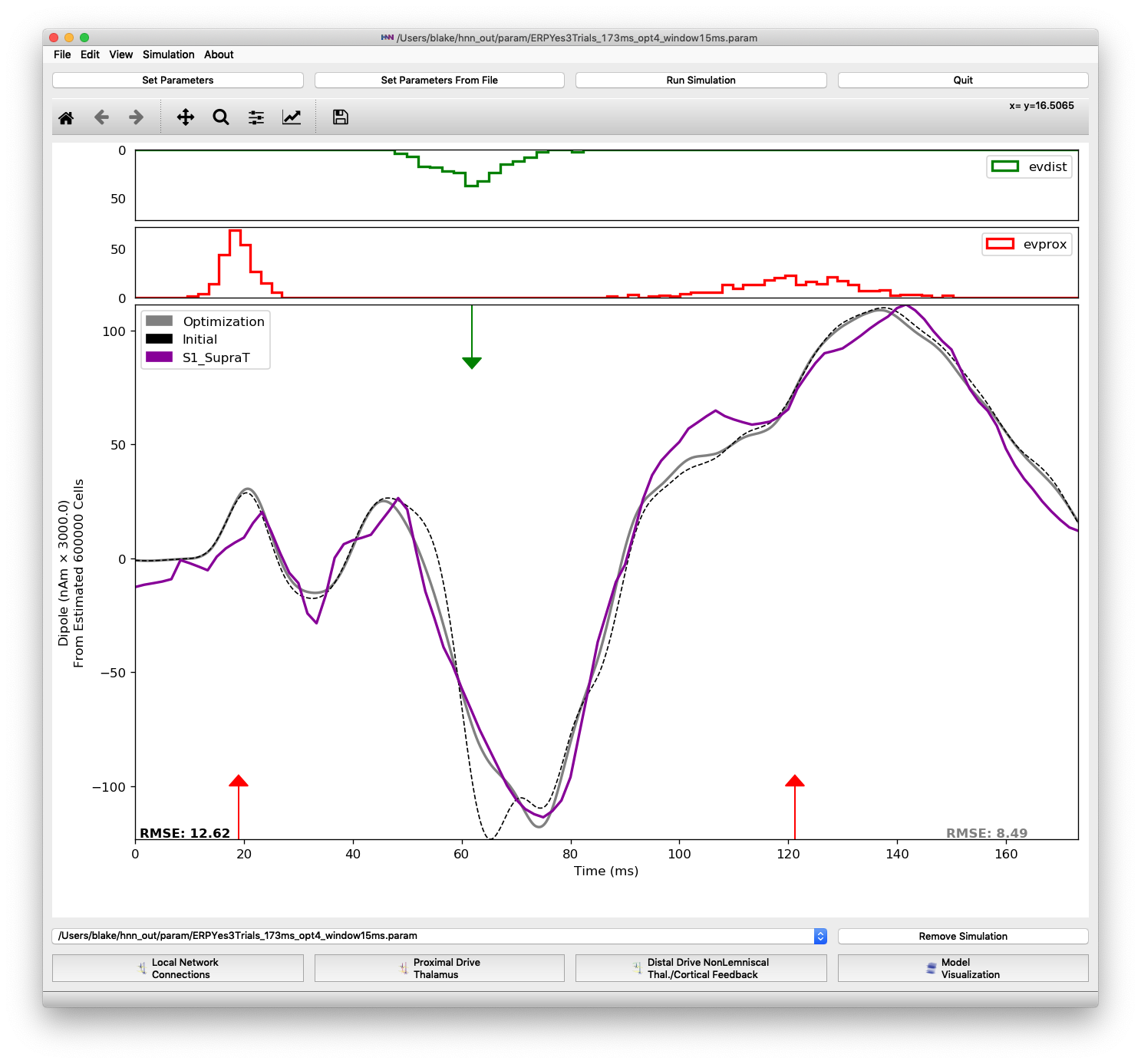
Fit after optimization using simulation trials with a 15 ms smoothing window
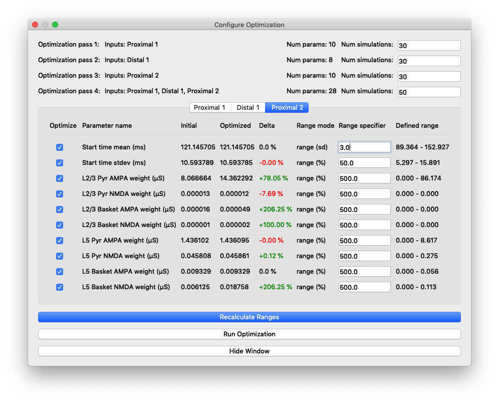
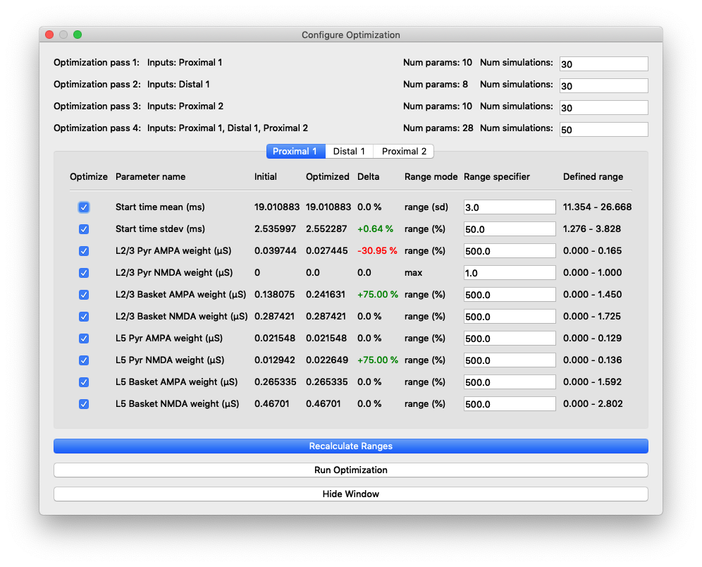
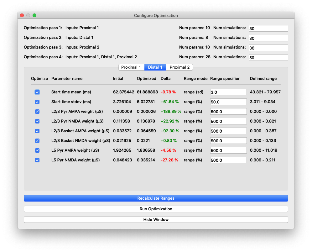
Note that there were minimal changes to the first and second proximal inputs. For those inputs changes were 75% or less, but for the distal evoked input, AMPA weights changed significantly. The plot reflects this in that the regions around the proximal inputs changed minimally, but the negative trough immediately following the distal input is fit very closely by the optimized parameters. The downward deflection follows the slope of the experimental data closely and nearly reaches its minimum at the same time, around 75 ms.
Through a total of 4 optimizations from a baseline parameter set designed for a different experimental scenario, we have found parameters matching new experimental data.
|
|

|
Parameter values and relative changes in the final optimization shown in Figure 12
Given our optimized fit plotting in Figure 11 and with parameters show in Figure 12, we can examine which parameters changed and by how much to form hypotheses on whether some parameters were more important to matching features. HNN’s GUI allows us to test these hypotheses by changing individual parameters and observing the differences in the dipole plots.
Below are examples where we worked backward from the optimized parameter values shown above (with RMSE 8.49) to identify the minimal parameters changes necessary to improve specific features of the ERP waveform.
For the region of the waveform immediately following the proximal 1 input, we found that increasing the L5 pyramidal NMDA weight was necessary to produce the second “bump” at 45 ms. Most of this change came about in the first optimization round where the parameter increased from 0 to 0.49. Figure 14 shows that changing the proximal 1 L5 pyramidal NMDA weight from 0 (dashed black line) to the final optimized value of 0.022649 (gray line).
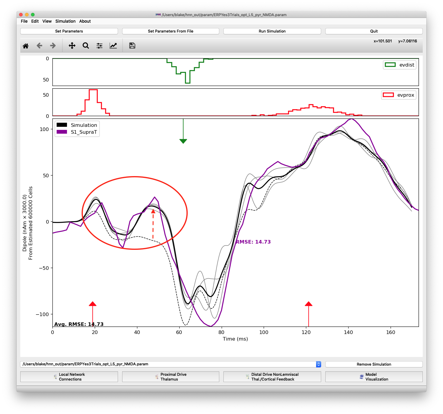
An increase in L5 pyramidal NMDA weighting (from 0 to 0.022649) results in a small peak at 45 ms.
Another parameter change necessary for matching features of the proximal 1 input was increasing L2/3 pyramidal AMPA and L5 basket NMDA weights. These changes contribute to the deep trough between 60 and 80 ms by pushing the dipole down as highlighted in Figure 15. Note that the optimized parameters for the distal 1 input are insufficient to produce the large negative dipole trough seen in the experimental data. Starting from an optimized fit, the values of these two parameters were changed to defaults, 0.01525 and 0.19934, respectively, to produce the dashed black line. Then optimized values were set, +80% and +134%, respectively, to produce the average of 3 simulation trials (solid black line)
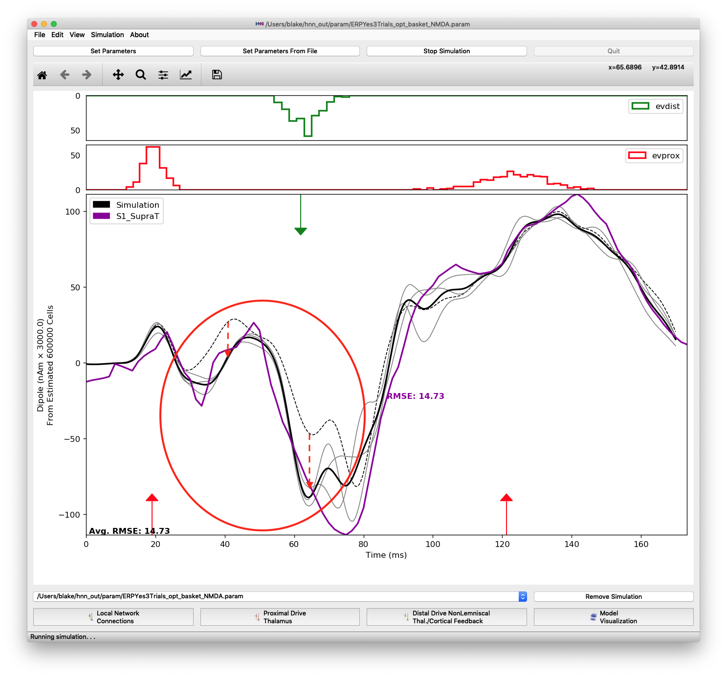
Difference when changing two parameters of the proximal 1 input: layer 2/3 pyramidal AMPA and layer 5 basket NMDA weights. These changes in the proximal 1 input are necessary to produce the trough at 75 ms. Changing the parameters of the distal 1 input alone is not enough to produce the trough.
For the distal input, the key parameters were the timing (mean start time and std. deviation) and the layer 2/3 pyramidal NMDA synaptic weight. During optimization the value for this weight changed repeatedly, increasing 31x from 0.0043 to 0.1369. Changing the timing and widening the std. deviation was necessary for matching the minimum and spread of the experimental dipole data at 75 ms. Figure 16 shows the optimized input for proximal 1 with only the three parameters changed for the distal input (layer 2/3 pyramidal NMDA, start time, and start time stdev). The RMSE dropped from 18.94 (dashed black line) to 13.55 for the partially optimized configuration (gray line).

Difference when changing 3 parameters of the distal 1 input: layer 2/3 pyramidal NMDA weight (31x), start time, and start time stdev. The dipole between 45 ms and 85 ms is shifted down by the NMDA parameter increase, while the minimum is shifted to the right by the timing parameters.
Similar to the previous inputs, only a few parameters of the proximal 2 input were significant contributors to the improved fit of features after the proximal 2 input. Besides decreasing the mean start time approximately 16 ms, increases in the layer 5 pyramidal NMDA and layer 2/3 pyramidal AMPA weights were necessary to push the dipole up to its maximum at 135 ms. The layer 5 pyramidal AMPA weight increased 110% and the layer 2/3 pyramidal AMPA weight increased 893%. The plot below shows the difference in changing the two synaptic weights. The dashed black line is from using default values for the proximal 2 input parameters (except mean start time of 121.2299) and the solid black line is from simulations using the optimized layer 5 pyramidal NMDA and layer 2/3 pyramidal AMPA weights, 0.0459 and 14.2738, respectively.
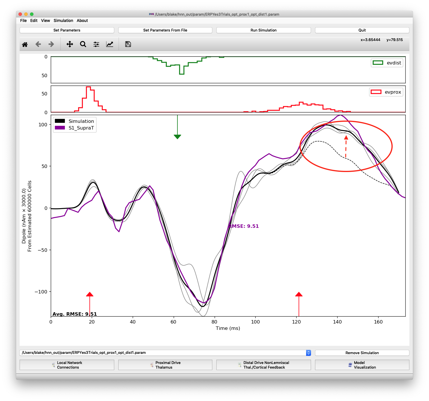
Difference when changing 2 parameters of the proximal 2 input: layer 5 pyramidal NMDA (+110%) and layer 2/3 pyramidal AMPA (+893%) weights. The dipole is shifted up following the last evoked input to more closely match the peak at 135-140 ms.
HNN includes a parameter file named “ERPYesSupraT.param” that is partially matched to the suprathreshold data used in this tutorial. Start an optimization from “ERPYesSupraT.param” and observe the differences in the optimized fit compared to the fit used in this tutorial. Is the optimization heading to a different fit than the one shown here?
The parameter file for the ERP elicited by non-detected stimuli “ERPNo100Trials.param” and data file “no_trial_S1_ERP_all_avg.txt” have dipole peaks and troughs with lower magnitude. The variability between trials is also greater using the “ERPNo100Trials.param” parameters. Try running an optimization using 10 trials (more than used for the suprathreshold-level optimization) and see if the RMSE for “ERPNo100Trials.param” can be improved upon. Is there a different set of influential variables for the non-detected stimuli scenario than the ones mentioned above for the suprathreshold scenario?
Neymotin, S. A. et al. Human Neocortical Neurosolver (HNN): A new software tool for interpreting the cellular and network origin of human MEG/EEG data. bioRxiv 740597; doi: https://doi.org/10.1101/740597
Powell, M. J. D. (1994). A Direct Search Optimization Method That Models the Objective and Constraint Functions by Linear Interpolation. In J.-P. Gomez Susana and Hennart (Ed.), Advances in Optimization and Numerical Analysis (pp. 51–67). Dordrecht: Springer Netherlands. https://doi.org/10.1007/978-94-015-8330-5_4